In Part 1 of this series I introduced the deep mathematics and impactful applications behind PDE-constrained optimization. If you’re interested in how this technology and its adjoint-based underpinnings work, be sure to check it out! Here in Part 2 I will go through the real-life problem of optimizing the yield of a chemical reactor. We will build a first principles model and then use PDE-constrained optimization to increase the so-called conversion ratio. I will provide lots of figures and hopefully a strong appreciation of the strength and breadth of PDE-constrained optimization!
The Reactor Model
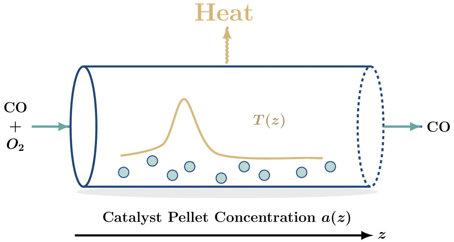
Let’s return to the gaseous $\text{CO}$ to $O_2$ converter, but in more detail this time. Figure 1 shows the physical setup. A mix of $\text{CO}$, $O_2$ and inert gasses (mainly N₂) enters the reactor on the left at a given inlet temperature $T_{in}$ and reacts via
\[2 \ \text{CO} + O_2 \to 2 CO_2\]The (local) reaction rate is given by the Arrhenius law –and is very sensitive to the local temperature $T(z)$ because the activation energy required to initiate the reaction is very high: $E_aa = 80,000 J / \text{mol}$. Here, $R = 8.314 J / (\text{mol} \ K)$ is the ideal gas constant and $k_0 = 10^{11} \text{mol} / (m^2 \ s)$ is the baseline reaction rate.
The incoming air molecules also have an average (superficial) velocity $u_g$. This velocity matters because when $u_g$ is high, most of the reaction will take place downstream. If $u_g$ is low, most of the reaction will happen at the inlet, increasing the chances of a dangerous temperature spike occurring.
As the $\text{CO}$ flows through the tube, it reacts on the catalyst pellets. The gaseous $\text{CO}$ is gradually converted to harmless $O_2$ and to solid carbon that stays at the bottom of the reactor. Increasing the amount of catalyst boosts the conversion but also raises the local temperature. The reaction is exothermic, so heat is released as $\text{CO}$ converts. Fortunately there are also two mitigating effects that counteract thermal runaway:
Excess heat leaves the reactor through its outer wall at a rate of $h_w [W / m^2 K]$. If $T_{\text{wall}}$ is the temperature of the reactor wall (here $500$ K), the local temperature inside will decrease at a rate of $h_w P/A (T(z) – T_{\text{wall}})$. Important is the cross-sectional perimeter-over-area ratio $P/A$. It indicates how much of the gas is able to lose heat. Typical cylindrical reactors have a small cross-sectional ratio, in fact, circles minimize it!
Diffusion transports heat across the reactor. Whenever there is a local temperature spike, that spike creates large temperature gradients and spreads out the particles, reducing the heat.
Governing Equations
The interplay of transport (convection), diffusion, reaction kinetics, and heat loss to the reactor wall fully determines how the system evolves. To capture this behavior, we track three key fields along the reactor:
-
$C_{\text{CO}}$, the concentration of toxic carbon monoxide
-
$C_{O_2}$, the oxygen concentration produced as a reaction byproduct
-
$T(z)$, the local temperature, which strongly influences the reaction rate.
Mathematically, the model is a set of three coupled convection-diffusion-reaction PDEs:
\[\begin{aligned} \frac{d}{d z}\left( u_g C_{\mathrm{CO}} - D_{\mathrm{CO}} \frac{d C_{\mathrm{CO}}}{d z} \right) &= - r_{\text{local}}(T, C_{\mathrm{CO}}, C_{\mathrm{O_2}}), \\ \frac{d}{dz} \left( u_g C_{\mathrm{O_2}} - D_{\mathrm{O_2}} \,\frac{d C_{\mathrm{O_2}}}{d z} \right) &= -\frac{1}{2}\, r_{\text{local}}(T, C_{\mathrm{CO}}, C_{\mathrm{O_2}}), \\ \frac{d}{d z} \left(u_g T(z)- D_T \frac{d T}{d z} \right) &= - \frac{\Delta H}{\rho C_p} r_{\text{local}}(T, C_{\mathrm{CO}}, C_{\mathrm{O_2}}) - \frac{h_w (P/A)}{\rho C_p}\, \bigl(T - T_{\mathrm{wall}}\bigr). \end{aligned}\]Let’s dig into what each of these equations represent. They follow directly from classical chemical reaction engineering. All three governing equations are written in flux form, which makes them easier to interpret. It is intuitive to imagine a small region around each point $z$. Each equation expresses a local conservation law: the rate of change of the total flux along the reactor must be balanced by sources or sinks due to chemical reaction or heat exchange.
The first equation represents $\text{CO}$ mas balance. $\text{CO}$ is transported downstream by the gas flow and simultaneously spreads due to diffusion with coefficient $D_{\text{CO}}$. These two terms together define the total flux of $\text{CO}$. As the gas flows through the catalust, $\text{CO}$ is consumed by the surface reaction at a rate $r_{\text{local}}$. The differential states that any decrease in the $\text{CO}$ flux in a tiny region must be exactly accounted for by the amount of $\text{CO}$ that reacts away within that region. The same applies to oxygen. It also travels to the right at speed $u_g$ and diffuses with coefficient $D_{O_2}$, but reacts away at only half the rate because two $\text{CO}$ are needed to react with one $O_2$ each species is transported downstream by convection at velocity $u_g$, spreads out by diffusion, and is locally consumed by the surface reaction.
The third equation represents energy conservation along the reactor. Thermal energy is transported downstream with the flowing gas and redistributed by heat dispersion. Note that, as the gas molecules flow, the associated temperature profile $T(z)$ will also move to the right. These mechanisms together define the heat flux. Energy is generated locally by the exothermic oxidation reaction. $\Delta H$ is the positive enthalpy released, $\rho$ is the gas density, and $C_p$ is its specific heat capacity. Heat is simultaneously removed through the reactor wall to the surroundings - proportional to the temperature difference with the wall. This is the last term in the thrid equation. The balance between these competing effects determines the temperature profile and causes phenomena such as hot spots and thermal runaway.
The catalytic surface reaction rate $r_{\text{local}}$ is harder to quantify because it depends on the precise atomic configuration. It is proportional to the probability that both a $\text{CO}$ and $O_2$ molecule occupy sites near a catalyst molecule. A classical macroscopic formula is the Langmuir–Hinshelwood rate law
\[r_{\text{local}}(T, C_{\text{CO}}, C_{O_2}) = k_0 \exp\!\left(-\frac{E_a}{R\,T}\right)\, \frac{ K_{\text{CO}}\, C_{\text{CO}} K_{O_2}\, \sqrt{C_{O_2}} }{ \left(1 + K_{\text{CO}}\, C_{\text{CO}} + K_{O_2}\, \sqrt{C_{O_2}} \right)^2}.\]Where we recognize the original Arrhenius reaction rate as the first factor, while the second factor comes from catalytic kinetics. Find out more about the Langmuir-Hinshelwood rate law here.
Temperature Spikes and Hysteresis
Before optimizing, let’s run some simulations of these partial differential equations – just to get a feeling for the sensitivity of the reactor to changes in the inlet temperature, and their effects on the ultimate conversion ratio. Figure 2 displays the temperature $T(z)$ and concentration of $\text{CO}$ throughout the reactor for two inlet temperatures: 750K and 800K.
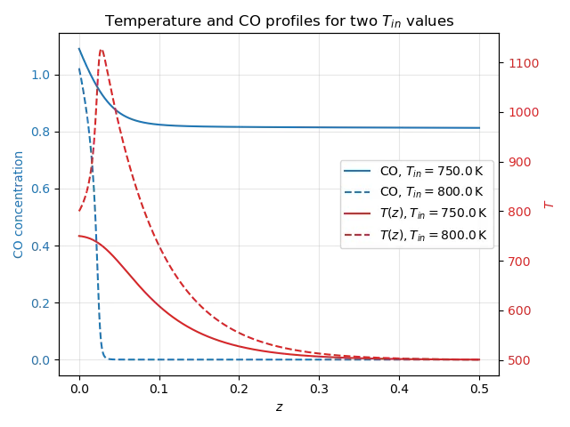
The total conversion ratio is about $13\%$, which is on the low side. Increasing the inlet temperature to 800K causes the reactor to go into thermal runaway, reaching over 1100K. The reason is essentially due to the Arrhenius law. A higher inlet temperature induces a higher reaction rate, and because the reaction is exothermic, it causes more heat to be released as $\text{CO}$ is converted. Increasing $T_{\text{in}}$ can have strongly nonlinear effects!
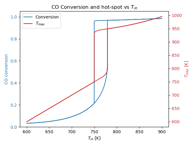
To explore how the reactor changes as we vary the inlet temperature, we can solve the PDEs for many different values of $T_{\text{in}}$ and keep track of both the maximum temperature and the conversion ratio. The resulting bifurcation diagram in Figure 3 reveals a sharp and abrupt transition. Above the critical inlet temperature (approximately 780 K), the system snaps into a thermal-runaway regime. The problem is even worse because of hysteresis: once the reactor is operating in the upper branch, we must cool it well below the critical temperature to return it into the safe zone.
Optimizing the Conversion Ratio
If we look at the lower branch more closely, we see that the conversion ratio can increase substantially before entering the upper branch. This raises a natural question: how much conversion can happen while keeping the reactor stable? This is exactly where the PDE-constrained optimization framework comes in.
Maximizing the conversion alone would push the optimizer straight onto the upper branch of the bifurcation diagram, with no mechanism to return to the safe operating regime. To avoid this, we must penalize excessive temperature increases: $T_{\text{in}}$ is allowed to increase just enough to boost conversion, while avoiding unsafe conditions.
Balancing these competing objectives leads to the following optimization criterion
\[\underset{a}{\min} \ J(a) = \frac{C_{\text{CO}}(\text{outlet})}{C_{\text{CO}}(\text{inlet})} + \gamma \int_{\text{inlet}}^{\text{outlet}} \max\left(T(z) - T_{\text{in}}, 0\right)\]In most setups, the inlet temperature is actually fixed. The optimization variable is the amount of catalyst $a(z)$ – which we assume constant along the reactor for now. Figure 4 shows the resulting bifurcation diagram as a function of a. The same hysteresis also occurs.
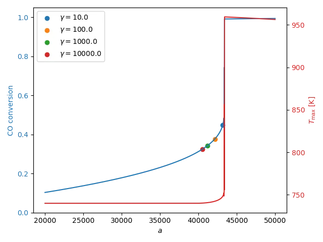
Let’s now turn to optimization. To keep things simple, we run a gradient descent algorithm on this objective. The method goes as follows. For each candidate $a$, we solve the PDE, evaluate the objective, compute its derivative using the adjoint method and pass both to the optimizer to update $a$. The optimization results for several values of gamma are also indicated on Figure 4. Their corresponding conversion and maximal temperatures are recorded in the table below.
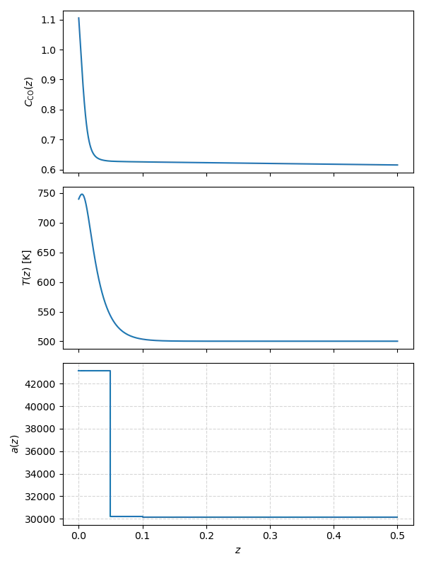
Large values of $\gamma$ impose a strong penalty on any temperature rise, keeping the temperature strictly under control. This avoid runaway but the resulting conversion of $32\%$ is on the low side. Reducing $\gamma$ to 10 relaxes the temperature constraint just enough to allow a modest rise above the inlet temperature, without entering the unsafe region – see also Figure 5. As a result, the conversion increases substantially, reaching $44.78\%$. This is precisely the increase in yield that we are interested, all through PDE-constrained optimization as a tool for optimal control! Note that the excess-temperature penalty is not strong enough to avoid runaway when $\gamma = 1.0$.
Multiple Catalyst Zones
A natural question is whether a spatially varying catalyst profile can do even better. We can run that experiment as well. We divide the reactor into five equal zones with catalyst concentrations $a_1, .., a_5$. The catalyst distribution now is piecewise linear. The gradient-descent optimizer can be extended to multiple dimensions, and FEniCS and Dolfin can easily handle five controls.
The optimized catalyst profile is shown in the final figure (Figure 5). The optimizer puts many pellets in the first zone, and a much lesser number in the other ones. The final conversion is essentially unchanged at $44.78\%$, but this design uses significantly less total catalyst, offering a clear cost benefit. We can explain why this is a near-optimal profile. Most of the reaction takes place at the inlet because temperature is highest there. As gas moves down the reactor, temperature decreases and it would not be beneficial to place many catalyst pellets, most would never react with the remaining $\text{CO}$.
Conclusion
PDE-constrained optimization is an underused tool in computational science – mainly due to its mathematical and numerical complexity. But many real-life control and design problems can be cast in this framework. We only need to ingredients: an objective function and an adjoint methods for computing its gradient. Modern finite-element packages like FEniCS provide these functionalities.
Here we successfully optimized the (financial) yield of a chemical reactor, but I strongly believe the most can be gained from this tool in topology optimization and the optimal design of shapes such as windmill blades, heat-conducting plates or even everyday kitchen utensils! Let me know if you’d be interested in a case like that.