Score-Based Generative Models for Uncertain PDE Solutions

In this project I explore Score-based Generative Models (SGMs) on a real problem in computational science. SGMs are the mathematics behind much of Generative AI (GenAI). I would argue that SGMs are the principled way of doing GenAI. Famous products like DALLE and Stable Diffusion rely on SGMs under the hood. Here, I apply it to an important problem in computational science: generating solution fields of PDEs with inherent uncertainty.

What are SGMs?

The idea behind SGMs is simple: given a bunch of samples ${x_k}_{k=1}^K$ from an unknown distribution $p_0(x)$ with $x \in \mathbb{R}^d$, generate new samples that are also distributed according to $p_0$. The way SGMs create new samples is complicated but principled.

My goal here is not to explain SGMs in all their glory, but rather to give a mathematical introduction sufficient enough to understand how they can be used in computational science. If you’re interested to learn more, I highly recommend you check out Jakiw Pidstrigach’s blog. He does an excellent job at explaining and motivating SGMs.

SGMs are based on stochastic differential equations, specifically the Ornstein-Uhlenbeck process and the backward Kolmogorov equation. Let $X_0$ be a stochastic variable distributed according to the data distribution $p_0(x)$. The Ornstein-Uhlenbeck process

has marginals $p_t(x)$ that converge to the standard normal distribution, i.e., $p_T(x) \approx \mathcal{N}(0,1)$ for sufficiently large $T$. Here, $dW_t$ is Brownian motion. Whatever the initial distribution $p_0$ is, the marginals $p_t$ will always become Gaussian after a while. Starting from a meaningful distribution we can always create noise.

Why is this important, or even relevant? The reverse-in-time equation (the backward Kolmogorov equation)

has the same marginals $q_s(x) = p_{T-s}(x)$. So, theoretically, if we initialize the backward SDE (2) with the standard normal Gaussian, we should obtain the original data distribution $q_T = p_0$. This suggests a simple algorithm: sample the standard normal Gaussian, simulate equation (2) using any timestepper, and you get new samples $Y_T \sim p_0$. This is the fundamental idea behind score-based generative models.

Looking back (pun intended) at equation (2), we need one crucial ingredient to simulate the Kolmogorov equation: the gradient of the logarithm of the time-dependent marginal $p_t$ of the forward problem (1). This is also known as the score. Unfortunately, no closed-form formula exists for this marginal, partly because it requires a closed formula for the data distribution $p_0$ (which we obviously don’t have). Instead, SGMs learn a neural network approximation to the score

where $\theta$ are the learnable weights and biases in the neural network. The input to the score network are stochastic particles, and the output is the local drift of equation (2). The score-network can be learned directly from the existing samples ${x_k}_{k=1}^K$, the training data, by minimizing the loss

That last equality is due to a theorem but it makes SGMs computationally feasible.

On $m_t$ and $v_t$ In practice, we never simulate the simple Ornstein-Uhlenbeck SDE (1) directly. Instead, we use a modified forward SDE

\[dX_t = -\frac{1}{2} \beta(t) X_t dt + \sqrt{\beta(t)} dW_t \tag{4}\]

with $\beta(t) = \beta_{\min} + t(\beta_{\max} - \beta_{\min})$. I.e., the forward drift opens up slowly as time increases. It can be shown that the invariant distribution of equation (4) is still the standard normal Gaussian, but the simulation and neural network training are much more stable with this modulated drift. Furthermore, the backward SDE now reads

\[dY_s = \frac{1}{2} \beta(T-s) \left(Y_s + s_{\theta}(Y_s, T-s)\right) + \sqrt{\beta(T-s) } dB_s\]

Finally, $m_t$ and $v_t$ are the mean and standard deviation of the conditional marginal $p_t(\cdot \mid X_0)$ and are given by

\[\begin{align*} m_t &= \exp\left(-\frac{1}{2} \alpha(t)\right) \\ v_t &= 1-\exp\left(-\alpha(t)\right) \end{align*}\]

with $\alpha(t) = \beta_{\min}t + \frac{1}{2} t^2 (\beta_{\max} - \beta_{\min})$.

A particularly useful flavor of SGMs are conditional SGMs, they learn the conditional data distribution

for many values of the conditioning parameter $z$. Conditional SGMs work in the same way as regular SGMs with one difference: the learned score function $s_{\theta}$ also takes $z$ as an extra input

That is, the network learns the score for many parameter values $z$ at once.

A Problem from Battery Design

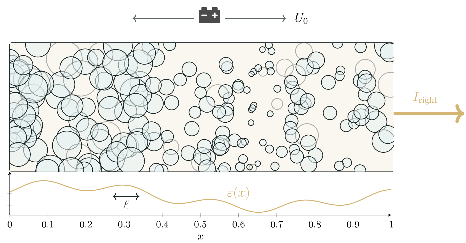
Modern batteries are porous, heterogeneous, active material full of electrolyte-filled pores and torturous pathways for ionic charge transport. The electric potential $\phi(x)$ and electrolyte concentration $c(x,t)$ inside the battery electrode are governed by two coupled and spatially heterogeneous transport equations. We assume the battery electrode is a narrow one-dimensional cylinder with height coordinate $x \in [0,L]$.

The coupled PDEs capture the interaction between electric transport in the electrolyte and interfacial electrochemical reactions at the solid–electrolyte interface. A crucial part in this complex interaction is the *porosity field $\varepsilon(x)$. The porosity measures how many holes are in the material at a certain location and how large they are. It is the main driver of physical uncertainty, yet determines $\phi$ and $c$ along with the macroscopic operating conditions. Figure 1 shows the porosity field inside the battery.

The electrolyte potential $\phi(x)$ is obtained by solving the quasi-static conservation law

Here, $k_{\mathrm{eff}}(x)$ is the effective ionic conductivity of the porous medium, $a_s(x)$ is the surface area density, $k_{rn}$ is a linearized reaction rate constant, $\phi_s(x)$ is the solid-phase potential, and $U_0$ is the equilibrium potential applied over the electrode. $U_0$ is an important macroscopic operating conditioning variable. The specific surface area is modeled as $a_s(x) = a_s^{(0)}\big(1 - \varepsilon(x)\big),$ which is where the porosity field $\varepsilon(x)$ enters the model: regions with less pore space (more solid surface) exhibit stronger volumetric reaction coupling.

The right-hand side represents a volumetric reaction current density, defined as

Reactions act as distributed sources or sinks of current in the electrolyte phase, coupling the electric potential directly to interfacial electrochemistry. Finally, the electrolyte concentration $c(x,t)$ evolves according to

Here, $D_{\mathrm{eff}}(x)$ is the effective diffusivity of the electrolyte in the porous medium, $t_+$ is the transference number, and $F$ is Faraday’s constant. The boundary conditions are what really drive this problem. The electric potential uses

corresponding to a no-flux condition at the left boundary and a prescribed ionic current flux at the right boundary. Since electric potentials are defined only up to an additive constant, the solution is normalized by enforcing $\phi(0)=0$ after solving. This is not an extra boundary condition but is necessary to make the solution uniquely defined. The electrolyte potential satisfies

corresponding to no-flux at the left boundary and a fixed concentration at the right boundary.

The Problem Statement The equations for $c$ and $\phi$ capture the essential coupling between the electric transport in a heterogeneous porous medium, the reaction kinetics at the solid–electrolyte interface, and ion mass transport. The steady-state solution $(c(x), \phi(x))$ is fully determined once the macroscopic operating conditions $U_0$, $F_{\text{right}}$ and the porosity field $\varepsilon(x)$ are known! That is, the model itself is fully deterministic. In any realistic setup, the porosity field $\varepsilon(x)$ is unknown. It depends on the exact atomic configuration of the electrode. Hence we must treat $\varepsilon(x)$ as an uncertain latent field, inducing a distribution over physically admissible solution profiles $\phi(x)$ and $c(x)$ under identical macroscopic operating conditions.

Training the SGM

The goal of this project is to train an SGM that can generate potential solution fields $(c(x), \phi(x))$ for given macroscopic operating conditions $U_0$ and $F_{\text{right}}$. In the language of SGMs, the samples are tuples $(c_0(x), \phi(x)) = X_0 \sim p_0$ and the score maps

Two important remarks about equation (6). First, the time coordinate $t$ is a purely internal time to the SGM and is not physical time in equation (^). In fact, we are only interested in steady-state solutions of the electrolyte concentration where all notion of time has disappeared. Second, we discretize the concentration and potential on a fixed grid before feeding it to the SGM. Concretely, we represent the 1D spatial domain $[0,L]$ by a uniform grid

and the unknowns / samples are vectors

We use $N=100$ grid points.

Training Data The training data consists of steady-state solution fields $(c(x), \phi(x))$ generated for a wide range of conditioning parameters. Because an SGM is trained to model a distribution rather than a single deterministic solution, it is essential to provide multiple valid solution fields for each fixed pair $(U_0, F_{\text{right}})$. In our dataset, we generate 100 distinct solution fields for each conditioning pair, across 250 different choices of $(U_0, F_{\text{right}})$ in total. The PDE solutions are computed using a second-order finite volume method.

The specific model parameters are $L = 10^{-4}$, $t^+=0.4$, $a_s=5 \times 10^5$, $k_{\text{rn}}=0.1$, and $\phi_s(x) = -1000 x$, and the effective conductivity and diffusivity are given by

with $\kappa_0 = 1.0$ and $D_0 = 3 \times 10^{-11}$.

Let’s finally talk about the distribution of the porosity field. We need to generate the training data from a known distribution, and then the SGM learns that distribution from the associated PDE solutions. We sample $\varepsilon(x)$ from a zero-mean Gaussian process on the grid with correlation length $l$. Afterwards, $\varepsilon(x)$ is scaled and shifted to fit inside the interval $[\varepsilon_{\min}, \varepsilon_{\max}] = [0.2,0.5]$ by

The sigmoid ensures the solution stays within this interval. In fact, we generate solution fields for many values of the correlation length $l$, so this becomes a third conditioning parameter

Neural Network Setup Since the score inputs are (discretizations of) continuous fields, the standard in SciML is to use convolutional neural networks. The input takes two channels (one for $c$, the other for $\phi$) of size $100$ and the output is another block with two channels, one for $\nabla_c \log p_t$, the other for $\nabla_{\phi} \log p_t$. In total, we use $20$ convolutional layers with $64$ channels and a kernel size of $7$. With a grid of $100$ discretization points, this means that any point should be able to ‘‘reach’’ any other point after $100 / 7 \approx 13$ convolutional layers. This means the network should be expressive enough. We use SiLU activation functions between the convolutional layers. No pooling is used because the input and output have the same size.

Conditioning is done through Feature-wise Linear Modulation (FiLM) layers. FiLM has shown tremendous potential as a tool for GenAI in visual reasoning. To the best of our knowledge, this is the first time FiLM has been applied in SciML. What is FiLM? A FiLM network is a simple MLP that modulates the output of the convolutional layers by scaling and shifting

Here $C_i$ is the output of the $i$-th convolutional layer (its size is $(B, 64, 100)$ with $B$ the batch size) and $(\gamma(p), \beta(p))$ are two vectors of size $100$ (also batched - so $(B,100)$). The FiLM layer multiplies the output feature-wise (or element wise), so the FiLM layer and to-be-modulated layer must have the same number of hidden features. The inputs $p$ are the conditioning parameters, in this case $p = (U_0, l, F_{\text{right}})$.

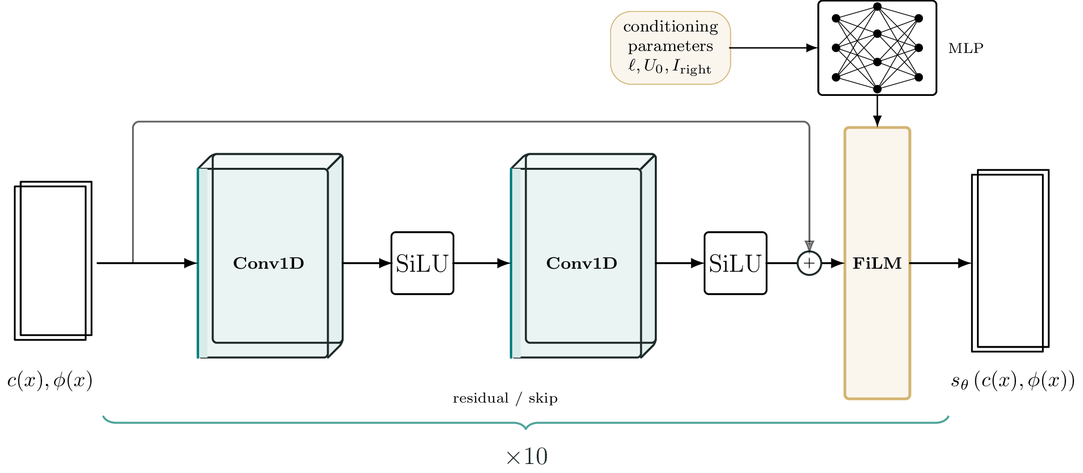
FiLM introduces incredible richness into the expressiveness of the score-based network. Our score-based network uses FiLM modulation after every two convolutional layers - so a total of $10$ FiLM layers. The total number of trainable parameters in the score network is 1.1M. This is probably way too many parameters for this problem, only five FiLM blocks would likely do, but we have not done any ablation studies yet.

Figure 2 displays one Conv-Conv-FiLM layer of our network.

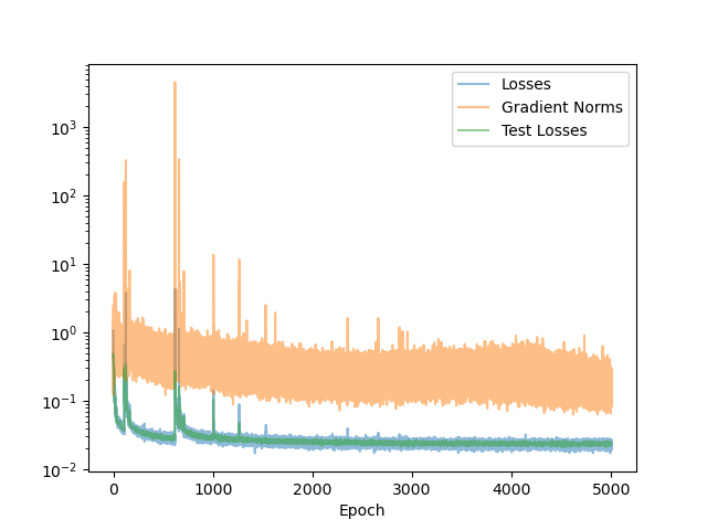
We train the SGM using the Adam optimizer with batch size $B = 1024$. The initial learning rate is $\eta = 2 \times 10^{-4}$ and we use a cosine scheduler to decrease the learning rate to $10^{-6}$ over $5000$ epochs. Figure 3 shows the training loss, loss gradient, and validation loss per epoch.

The Sampling Results

SGMs should agree in distribution with the underlying PDE. Unfortunately, we cannot compare the finite-volume simulation for a given porosity field $\varepsilon(x)$ with the output of the SGM because the SGM never constructs $\varepsilon(x)$ explicitly - it is inaccessible. Instead, we can compute the mean, variance and percentiles of both distributions and see if they match.

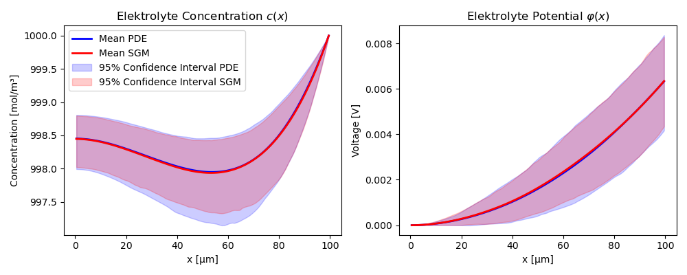
Figure 4 shows the average solution fields $c(x)$ and $\phi(x)$ of $1000$ realizations of $\varepsilon(x)$ for both the PDE and SGM for fixed operating conditions $U_0 = 0$ and $F_{\text{right}}= 25$. We also plot the 95\% confidence interval around this mean. Clearly, the SGM is unbiased and captures the uncertainty of the distribution very well! Even more, we can see the confidence bounds collapse near Dirichlet boundary conditions ($\phi(0) = 0$, $c(L) = c_{\text{right}}$) and we also see the no-flux boundary condition at $x = 0$ for $c$. Again, the porosity field $\varepsilon(x)$ is never passed to the SGM - it learns its distribution.

My Outlook on the use of GenAI in Computational Science

Score-based generative models are a good example of what I find genuinely exciting about generative AI for scientific computing. Not because they solve PDEs, but because they generate distributions of physically plausible solutions. This is a crucial part of much current research in uncertainty quantification. SGMs give us a way to represent uncertainty and variability in a data-driven yet principled way.

At the same time, I am slightly skeptical of using GenAI as a blunt replacement for numerical solvers or first-principles modeling. For example, traditional PDE solvers have known 50+ years of progress and improvements and are unbeatable in speed and accuracy. Modern paradigms like physics-informed learning have not been around long enough to be a serious contender. What works well is using generative models as a component in a larger computational pipeline: as fast proposal mechanisms for Bayesian inference for ill-posed inverse problems, as surrogates for expensive micro-scale solvers, or as ways to explore the space of feasible physical designs or states before fine-tuning with advanced, accurate but very slow traditional solvers.

More broadly, I think the real promise of GenAI in computational science is to alleviate bottlenecks and numerical kernels. Generative models offer a way to soften these bottlenecks by learning enough of the macroscopic structure from data and encoding it in a form that is easy to sample, evaluate, and differentiate; and integrate into existing numerical pipelines. I believe GenAI can turn previously intractable uncertainty quantification into something that becomes computationally feasible - like I tried to demonstrate in this example.

GenAI and SGMs are new tools in the ever expanding computational toolbox; the key is to use them for the right problem. The most impactful applications will likely come from hybrid approaches: physics-informed generative models, generating good initial guesses for expensive numerical routines, and sampling stochastic models. I hope this project is one small step in the direction of a broader computational science and SciML workflow.