A Physics-Informed Neural Operator for Newton's Heat Law

I recently started a project to understand physics informed neural networks (PINNs) and operators (PINOs) better. My goal is to train a physics-informed neural operator for a second-order PDE in three dimensions with non-trivial boundary conditions. Read more about my plan and my ultimate goal in my previous post. Today, we begin the first leg of this journey: learning the time-dependent solution to Newton’s heat law for any input time and combination of model parameters.

Newton’s heat law describes how the temperature of an object changes when the object is put in a heat bath. Let $T(0) = T_0$ be the initial temperature of the object, and let the surrounding heat bath have a fixed temperature $T_s$. The object’s temperature will converge towards $T_s$ with rate $k$ which is given by the object’s surface area, heat capacity, and microscopic structure. In general, temperature $T(t)$ at time $t$ satisfies the (ordinary) differential equation

We assume that the temperature is uniform throughout the object. If not, we would need to model the spatial temperature profile using a partial differential equation, but that would lead us too far. Equation (1) is simple enough that we can immediately write down its exact solution

The temperature decays exponentially from $T_0$ to $T_s$. In total, there are three free parameters: the initial temperature $T_0$, the heat bath temperature $T_s$ and the rate constant $k$. The object’s temperature as a function of time, $T(t)$, depends on all three. Physics-informed operators should have no problem modeling the exponential decay as a function of three parameters. Let’s dig in.

A Simple PINO

Our first physics-informed neural network takes time $t$ and the three parameters as input. The output is just the current temperature $T(t)$. We start with the simplest setup imaginable: a simple multilayer perceptron (MLP) with two hidden layers and $z=32$ features per layer.

The loss function is what differentiates PINNs from other types of networks. For an input batch ${t_b, k_b, T_{0,b}, T_{s, b}}$ of size $B$, it is standard to use the 2-norm of the physics residual as the loss, i.e.,

This formulation works fine theoretically, but our training data will consist of many orders of magnitude for the rate constant $k$. When $k$ is small, the temperature will decay slowly, for large $k$, the temperature will converge to $T_{s,b}$ very quickly. It therefore makes sense to cast everything into unitless time $\tau = k t$. The make the loss of similar order for all input parameters $k_b$,

Making time unitless is one of the most important aspects of getting PINNs right. Hence we will also use it as the fundamental time input.

What about the (Dirichlet) initial temperature $T_0$? It is also standard in the PINN literature to incorporate any Dirichlet boundary conditions directly into the network output. Otherwise, one would need to add a second term to the loss function. Both work in theory, but mixed optimization is much, much more difficult in practice. Let $g_{\theta}(\tau_b; k_b, T_{0,b}, T_{s,b})$ represent the trainable part of our formulation, the complete neural network output is

When $\tau = 0$, the Dirichlet boundary conditions are automatically satisfied and the network tries to learn what happens when $\tau > 0$. This is a good first setup.

Before showing the results, let’s talk about the training data. If this PINO is really meant to understand physics, the training data $(t, k, T_0, T_s)$ should span a wide and representative range of possible regimes. In particular, we sample $\log k$ and $\tau$ instead of $k$ and $t = \tau / k$ respectively. Relaxation rates $k$ typically vary over orders of magnitude, and uniform sampling in $k$ would heavily bias the dataset toward fast dynamics. Sampling in log-space ensures balanced coverage of both slow and fast regimes, allowing the network to learn the correct scaling behavior across time scales instead of overfitting. In this example, we sample $\log k$ uniformly between $\log(10^{-2})$ and $\log(10^2)$. Regarding training data for time $t$, Newton’s heat law fundamentally only knows $\tau$, so we might as well lean into it. We sample $\tau$ uniformly in $[0,8]$. Finally, we sample the initial and final temperature $T_0$ and $T_{s}$ uniformly in $[-T_{\max}, T_{\max}]$ with $T_{\max} = 10$.

A Note about Normalization

Independent of PINNs, we must also normalize the data before feeding it to the network. Normalization typically ensures that data has zero mean and unit standard deviation, or that it lies within the interval $[-1,1]$. In our case, this amounts to normalizing $T_0$ and $T_s$ by dividing by $T_{\max}$, normalizing $\log k$ by dividing by $\log(10^2)$, and normalizing $\tau$ by dividing by $\tau_{\max}=8$.

In summary, the complete input-to-output relationship reads

The trainable parameters, weights and biases, are collected in $\theta$.

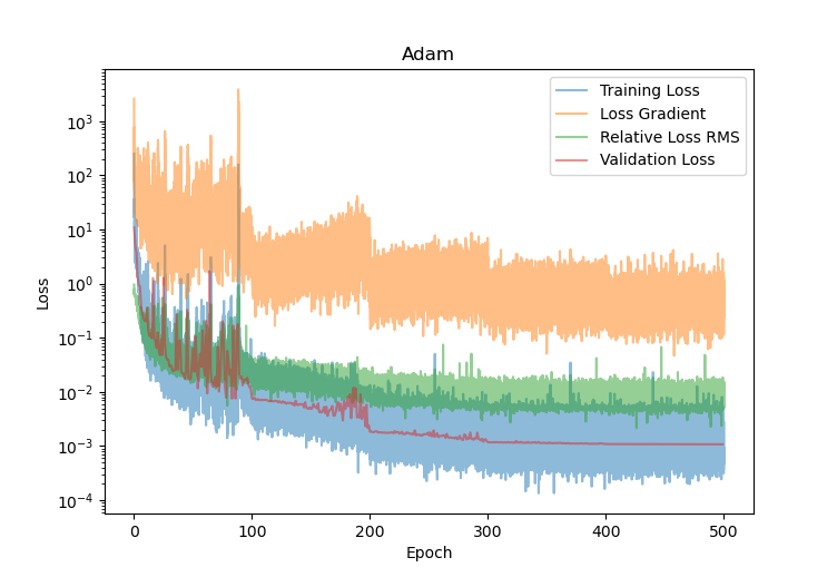
We train this neural network with the Adam optimizer. The learning rate starts at $10^{-2}$ and decreases by a factor $0.1$ ever $100$ epochs. The batch size is $B = 128$, very standard in the PINN literature. The loss, loss gradient and validation loss are shown in Figure 1. Clearly, the loss is decreasing steadily, and the validation loss follows the same path. The PINO is actually learning! The loss gradient is large but also decreases more steadily. A large gradient is not by itself a problem: the PINN loss involves the temperature derivative, which can be noisy, so the basin of tiny loss might simply be very narrow.

Another useful metric to plot is the relative root mean-squared error (RMS) of the loss, defined by

This relative error should decrease significantly over the course of training. It is an indicator that the neural network is learning the physics. We see on Figure 1 (green curve) that it indeed does.

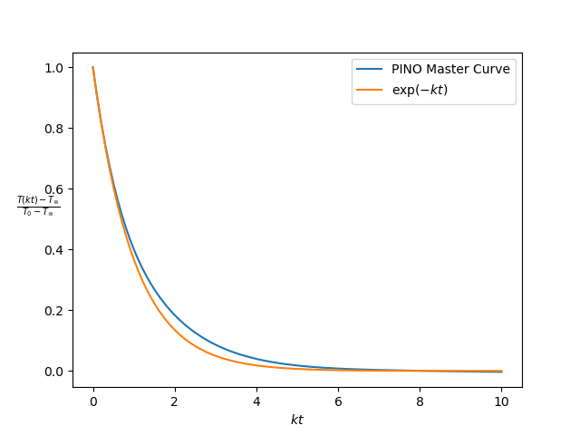
Training and validation loss and relative RMS by themselves are useful convergence metrics, but they don’t tell us anything about how well the PINN performs on independent test data. We are interested in calculating the actual temperature profile $T(t)$ for any initial temperature $T_0$, bath temperature $T_s$ and rate $k$. Fortunately, we can compare this profile with the analytic solution (Equation (2)). Figure 2 (left) shows a comparison for an unseen test parameter. The temperature profile follows the initial exponential profile, but there is a large and constant bias for large $t$. We can measure this bias by considering

This equation represents an invariant of the physics. Invariants reduce the effective dimensionality of the mapping $t \mapsto T(t)$. The PINO should reproduce this ‘master curve’, i.e.

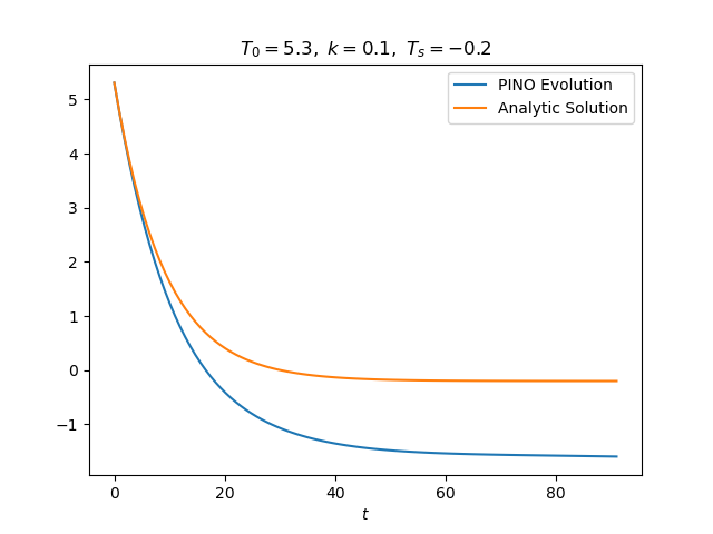
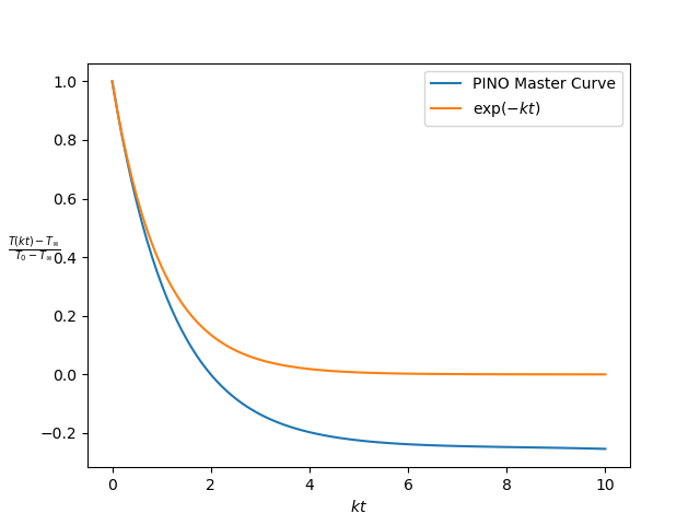
Figure 2 shows the PINO clearly learned something about the exponential decay, but there is a large bias for large $\tau$. What could be the reason for this bias? What is going wrong here?

Being more careful about the Dirichlet Boundary

I was initially puzzled by this bias. It looks like a bug in the code: a wrong factor or perhaps we’re just computing the master curve wrong.

However, the problem is more insidious. Looking back at the formula for the predicted temperature (Equation (3)), the factor $\tau$ is a problem. Sure, when $\tau$ is zero, the Dirichlet boundary condition is satisfied. But what happens as $\tau$ grows? The trainable function $g_{\theta}$ needs to essentially learn a $1/\tau$ factor. Inverses are tough for any neural network. This problem is perfectly fixable once you realize that the prefactor does not need to be $\tau$ exactly. Any function of $f(\tau)$ will get the job done as long as $f(0) = 0$. Ideally, $f(\tau) \to 1$ as $\tau$ grows. We use

Note the extra factor $2$. We could just make it easy for ourselves by using the exact time decay $1-\exp(-\tau)$ as a prefactor (see Equation (2)), but that would be disingenuous. I want to learn as much as possible about physics-informed learning, so let’s make it intentionally harder. Training is now a lot more difficult than it should, but Newton’s law is so simple that a PINN should be able to deal with this explicit bias.

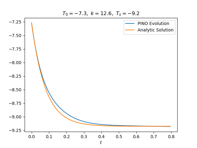
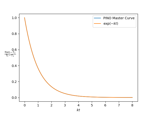
With the introduction of this exponential time factor, we get a much better approximation of the master curve - see Figure 3. The bias for large $\tau$ is completely gone; the PINO even learned to correct for the explicit bias in the time factor for small $\tau$! The example on the right tells the same story.

The Secret Sauce: L-BFGS for Fine Tuning

Adam is a great all-purpose optimizer and should essentially always be used to bring the initial loss down many orders of magnitude. However, on its own it will never be enough to learn the fine detail of a physics-informed neural network or operator; especially when the physics gets harder. The reasons are twofold: the loss function and batching. First, the loss depends on the derivative of the neural network output. A slight change in inputs $t$ or $\tau$ will cause a relatively large change in $T(t)$ and its derivative $dT(t)/dt$. The local minimum in the loss where the physics is satisfied is narrow and Adam will never be able to fine-tune the weights enough to hit the bottom of the loss well. Batching exacerbates this problem. The Adam optimizer follows the local loss gradient to propose a new set weights. With batching, the local gradient is random and Adam will bounce around the local minimum in parameter space without ever reaching it.

L-BFGS improves convergence to the loss minimum on both counts. Although it is almost never explicitly mentioned in the physics-informed literature, L-BFGS is always used to fine-tune the loss. Most of the time, we can reduce the loss by many more orders of magnitude! Why does L-BFGS improve convergence? First, the search direction is not the local gradient but something that resembles the Newton search direction. It can be shows that the newton direction ($-H^{-1} \nabla_{\theta} \mathcal{L}$ with $H$ the Hessian) generally points in the direction of the local minimum. An additional line search step guarantees the biggest loss decrease along this search direction. Second, unlike first-order optimizers, L-BFGS works on the full dataset at once, or a deterministic subset of it, not on random batches. A full explanation of L-BFGS would lead us way to far, let us just show the final results for now.

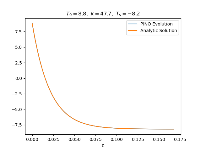
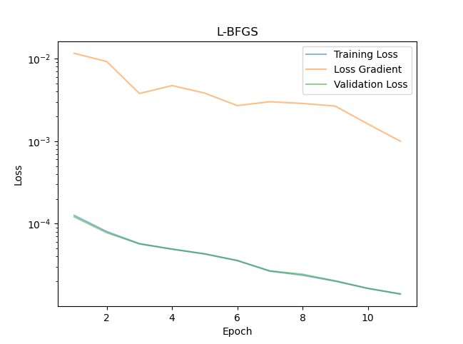
So how does L-BFGS perform? Starting from the final Adam checkpoint, we see in Figure 4 that the loss decreases to $2 \times 10^{-5}$. Furthermore, Figure 5 displays a much better approximation to the exponential decay!

Conclusion

This first step was already much more interesting and complicated than I thought. What started as learning the solution to a simple ODE quickly bifurcated into side quests about biased sampling, time biasing and higher-order optimizers. I learned a lot and we’re one step closer to my goal!

Here are the things I learned:

• Incorporate as much of the known physics as possible in the neural network output. Here, we essentially trained the neural net in dimensionless time units ($\tau$) - already a big regularization!
• Always encode Dirichlet boundary conditions directly in the neural network output, but be careful about the form of the time factor! A linear factor is not great because it forces the network to learn a $1/\tau$ multiplier.
• Normalize all inputs and outputs to have a zero mean and unit standard deviation or lie in $[-1,1]$. Normalization is essential because most of the nonlinearity in the activation function happens near $0$.
• The Adam optimizer is great to start training because it reduces the initial loss to an acceptable regime, but L-BFGS is necessary to obtain a close approximation of the true solution.

I will remember these lessons as I embark on the next leg of this journey: learning a PINO for the full heat equation. Stay tuned!