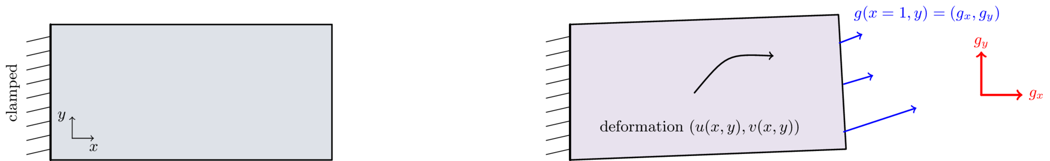
Our first 2D example with traction boundary conditions

I’ve been exploring Physics-Informed Neural Operators (PINO) over the past two months. Starting from a simple equation, Newton’s heat law, we trained a PINO to predict the temperature evolution given any initial temperature, heat bath temperature and rate constant. We have been steadily increasing complexity of the underlying physics, culminating into a complete neural operator for solving the heat equation: a partial differential equation in space and time where the initial condition is a function in space. Read about this journey in my previous blog posts: A Physics-Informed Neural Operator for Newton’s Heat Law, Learning the Heat Equation, Operator Learning: The Right Way and The Deep Truth about Physics-Informed Learning!

The heat (or diffusion) equation is an interesting model for studying numerical methods. Temperature decays exponentially and its rate depends only on the diffusion constant. However, the equation is too simple: solutions will always be decaying exponentials, no other solution forms are possible. In addition, we only used Dirichlet conditions in the form of fixed initial and boundary temperature (profiles). In this post we move to a more complex equation: linear elasticity in two spatial dimensions with traction boundary conditions!

Elastodynamics is deeply personal to me; it’s where I first fell in love with computational science. As an engineering undergrad, I spent my summers using finite element methods to hunt for cracks in materials by tracking wave propagation. In three-dimensional linear elasticity, waves ‘focus’ at material discontinuities—effectively lighting up the very cracks we were looking for. About a year ago, I revisited this model by training Physics-Informed Neural Networks (PINNs) for linear elasticity and … failed. Only last week did the missing pieces click. After a bit more coding, debugging, increasing performance, and getting frustrated with AI tools, I’m finally ready to share the results. I hope you find it interesting!!

The Linearly Elastic Regime

Many solid objects deform when forces are applied to them. A metal plate, for example, may bend, stretch, or shear slightly when it is pushed or pulled along its boundary. In mechanics, one of the simplest and most useful models for describing this behavior is the theory of \emph{linear elasticity}. This theory applies when the deformations are small, meaning that the object changes shape only a little compared with its original size. In that case, the relation between the applied forces and the resulting deformation can be approximated well by linear equations.

The working example for this post is a thin metallic plate. Because it is thin, we can essentially think of it as two-dimensional with domain $\Omega=[0,1]^2$. Before any force is applied, the plate is flat and undeformed. This initial state is shown in the left pane of Figure 1. We describe the deformation of the plate by a displacement field $(u(x,y),v(x,y))$, where $u$ is the horizontal displacement and $v$ is the vertical displacement. In other words, if a material point starts at position $(x,y)$, then after deformation it moves to $(x+u(x,y),\,y+v(x,y))$.

The left boundary of the plate, located at $x=0$, is clamped to a rigid wall. This means that the plate is fixed there and cannot move. On the opposite boundary, at $x=1$, a traction force is applied

This traction is not applied at a single point; rather, it acts along the entire right boundary. A good mental picture is a liquid streaming against the wall: the water touches the boundary everywhere, not just at one point. The components have a simple interpretation: $g_x(y)$ describes how strongly the boundary is being pushed or pulled in the horizontal direction, while $g_y(y)$ does the same in the vertical direction. The effect of this loading is shown schematically in the right pane of Figure 1. Once the traction is applied, the plate deforms, and that deformation propagates throughout the material. Depending on the form of $g_x$ and $g_y$, the plate may stretch, compress, or shear.

The amount of deformation and shearing is partly determined by two material constants: The Young modulus ($E$) and the Poisson ratio ($\nu$). The former measures the intrinsic resistance to stretching in the material: high Young modulus means a lot of energy is required to extend the material, a low Young modulus indicates the opposite. On the other hand, the Poisson ratio measures how much the ‘$y$’ direction can ‘tighten’ if we pull on the other ‘$x$’ direction.

We work in the linearly elastic regime, which means that we assume the deformations are small and that the material behaves elastically. In this setting, $E$ and $\nu$ fully determine how a material will deform under any load. Our goal is therefore to predict this displacement field $(u,v)$ produced by a given boundary traction $(g_x,g_y)$.

In static equilibrium, the total force acting on every small piece of material must vanish. The equilibrium deformations can be described by the partial differential equation

This equation expresses a local balance of forces: internal elastic forces, represented by the stress tensor $\sigma(u,v)$, must balance any external force density $F(x,y)$ acting inside the material. Don’t be discouraged by the term tensor, it is just a fancy word for a matrix (purists will disagree).

Let’s go through the terms and symbols. First, $\sigma(u, v)$ is the stress due to displacements $u(x,y)$ and $v(x,y)$. The stress tensor $\sigma(u,v)$ describes the internal forces generated by the deformation of the plate. In two dimensions, it is a $2 \times 2$ matrix

The stress matrix is the only place where these material parameters will show up. Also, subscripts $x$ and $y$ indicate derivatives, so

The operator $\nabla \cdot \sigma$ is the divergence of the stress tensor. It converts internal stresses into a vector of net internal force. If the stress varies from one point to another, then those variations produce a resulting force on a small piece of the material. Equation 1 states that this internal force must be completely balanced by the external body force $F$.

In our case, there are no forces acting in the interior of the plate. So $F(x,y) = 0$ in the bulk of the material. All forcing $(g_x, g_y)$ is applied to the boundary of the material. Let’s talk about the boundary conditions some more. The left edge of the plate is clamped, so that

so the material is unable to move. On the right edge we prescribe the traction

where $\overrightarrow{n}$ is the outward unit normal vector. For the right boundary, $\overrightarrow{n}=(1,0)$. These boundary conditions correspond exactly to the physical situation shown in Figure 1: the plate is fixed on the left and loaded on the right by a distributed boundary force. Strictly speaking, this is a traction boundary condition rather than an ordinary Neumann condition, but it plays a similar role: it prescribes boundary data for the stress tensor, which depends on first derivatives of the displacements.

The top and bottom edges corresponding to $y=0$ and $y=1$ are free boundaries; no force is applied there. That is,

I didn’t know for the longest time that you actually need to prescribe these boundary conditions to the code and physics - realizing this was the breakthrough to training the PINO!

Learning Deformations

The linear elasticity equation (1) can be directly used in the physics-informed loss term by squaring it. However, evaluating the loss is very slow because it involves second-order derivatives: one order coming from the stress tensor and another from taking its divergence. Especially in two or more dimensions, evaluating second derivatives is a real bottleneck. The main reason is the size of the computational graph that needs to be constructed in memory. This graph is still manageable for the first derivative - like backpropagation / AD to the network weights - but blows up for the second derivative because it includes the graph for the first derivative as well. PyTorch has some great vectorized functions like jacrev and vmap to make these computations faster, but there is no avoiding the need for RAM memory. Especially with prices skyrocketing, there must be another way.

One nice feature of linear elasticity is that it has an energy principle. It can be shown that the partial differential equation (1) is equivalent to minimizing the potential energy

where the coefficients are given by $C_{11} = E/(1-\nu^2), C_{12} = E \nu/(1-\nu^2), C_{66} = 0.5 E / (1+\nu)$, and $\partial \Omega_N$ is the boundary where the traction is applied ($x=1$ in our case). The top and bottom boundaries are free, so their traction is zero and contribute zeros to the energy.

Think of a material as being made up of tiny microscopic springs. We can describe the deformation of a spring on two levels: the forces acting on it according to Newton’s law, or the energy that is contained in the spring. Both descriptions are equivalent. The linear elasticity PDE (1) is the first approach, while the energy principle (2) is the second. In fact, the coefficients $C_{11}, C_{12}$ and $C_{66}$ come from writing Hooke’s law in two dimensions!

Minimizing (2) has two advantages in the context of physics-informed learning. First, the potential energy only contains first derivatives of $u$ and $v$, which makes evaluations much cheaper than the residual of (1), and by extension training the PINO. Second, we can directly use the energy as the loss function. No need to residualize it, the potential energy is the loss! The only downside that I can think of is that the energy can be negative. In fact, the optimal potential energy will have some negative value. Negative losses are not a problem for gradient-based minimizers, it just makes the loss harder to interpret for us humans. Not unrelated, the loss naturally scales with the magnitude of the boundary forcing $g$. If the training set is resampled at every epoch, the loss will jump around, making it harder to assess convergence. It is therefore very important to rescale the energy by $\lVert g \rVert$, because only then will a decreasing energy be a sign of convergence.

The only remaining question is how to evaluate the integrals in equation (2) numerically. Our PINO approach takes in grid points $(x, y)$ and forcing functions $g$ and outputs point estimates of the displacement field

In the ‘strong’ setting one would just evaluate equation (1), compute its residual, and sum over the batch. In our ‘weak’ sense, the loss is an integral over the complete domain $\Omega$ and its (traction) boundary $\partial \Omega_N$. This means we need to propagate a whole batch of $(x_i, y_i)$ samples (for a given boundary forcing) for one loss or energy evaluation. In fact, we need to propagate two batches of samples: $\left{x_i, y_i\right}{i=1}^N$ for the bulk $\Omega$ and $\left{y_j\right}{j=1}^M$ for the boundary $\partial \Omega_N$. Fortunately, any classical numerical integration method works fine in our context. I use a Monte Carlo method with 5000 random points in the bulk, sampled every epoch. Monte Carlo induces some extra noise in the loss evaluations, but reduces the risk of overfitting on a fixed quadrature grid.

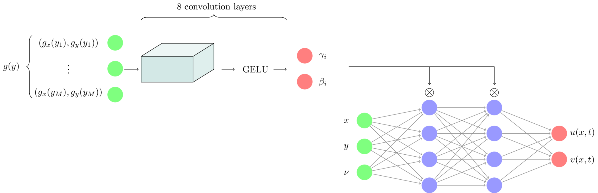
The Neural Architecture

The neural architecture is very similar to the one we used for the diffusion equation. Borrowing the terms ‘branch’ and ‘trunk’, the input to the branch network are the boundary forcing functions $g_x$ and $g_y$ on a fixed grid of $101$ points. For each training example, we sample the two components as independent Gaussian process on $y \in [0,1]$ with zero mean and correlation length $l = 0.2$. This produces smooth random traction profiles. Have a look at Operator Learning: The Right Way if you want to see a pretty picture of these boundary forcing functions.

The branch network consists of $8$ convolution layers where the number of channels increases gradually from $2$ (one for $g_x$ the other for $g_y$) to $64$. We combine all channels at the end by average pooling. The branch network uses Feature-wise Linear Modulation (FiLM) to attenuate the hidden layers of the trunk network.

The trunk network is a simple Multilayer Perceptron (MLP) with three inputs $(x, y, \nu)$ and two outputs $u(x,y), v(x,y)$. Each hidden layer has $64$ neurons, and the output of each layer, $h_i$ is modulated by the FiLM coefficients $\beta_i$, $\gamma_i$ element-wise

before being passed through the nonlinear activation function (GELU). The total number of trainable weights is about 300,000. Figure 2 shows the complete architecture of this neural operator.

The Young modulus is not an input to the neural network. The reason is that the solution to the linear elasticity PDEs (1) scales linearly with its inverse $1/E$. Indeed, increasing the stiffness $E$ by a factor of $10$ reduces the displacement field by the same factor for identical forcings. Equivalently, to produce the same displacement in a material that is ten times stiffer, one must also increase the applied traction by a factor of ten. In that sense, the physically relevant input is not the raw traction $g(y)$, but rather a scale-invariant forcing obtained after normalization by $E$. In fact, the Gaussian process generates scale-invariant sample traction functions. One of the lessons we learned is that including more physics into the network output improves the PINO. Adding scale-invariance to the network is very much in this spirit.

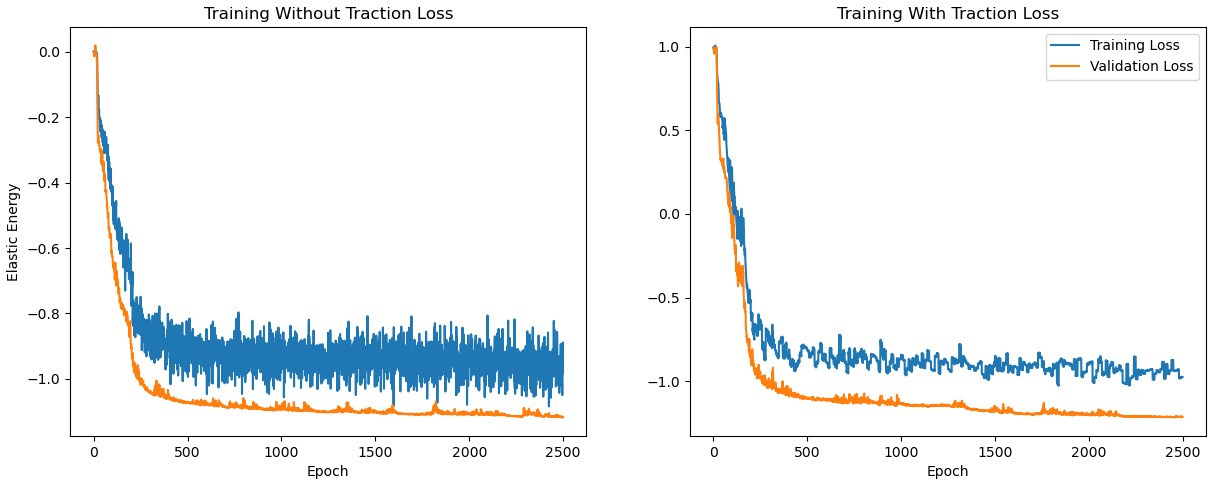
Training this network was not straightforward. We found that adding a pure traction-loss with a small weight tremendously improved convergence. The traction loss is of the form

making the full physics-informed loss

This extra boundary-traction loss is really what makes the network initially converge. Even with $\lambda = 0.1$, training progresses much more smoothly, and the final loss is much lower. Figure 3 compares the training scenarios without and with extra traction loss. The main difference is the speed of initial loss decrease and the noise level during training.

I want to emphasize that adding a traction loss is still physics-informed learning, the idea is just slightly less beautiful than the energy formulation (2) alone.

Some Pretty Pictures

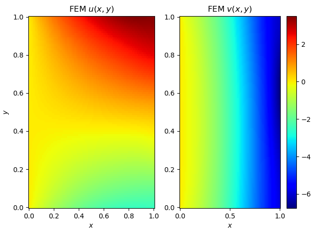
Figure 4 compares a sample displacement field generated by our PINO with the corresponding finite element solution of the linear elasticity problem, computed on a similarly sized mesh and for the same boundary forcing. We observe close agreement, both in the global deformation behavior and in the finer structural details.

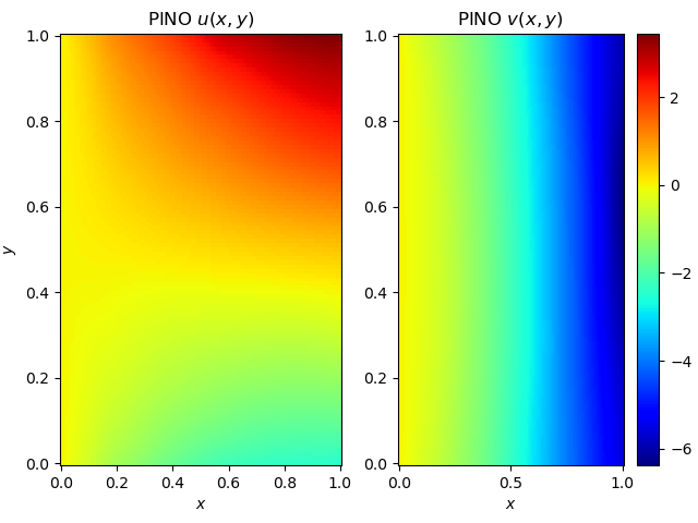
More importantly, these figures are a testament to the beauty that can be created by computational science (corny, I know…).

What’s Next?

Writing this post was another deeply personal experience for me. I’ve finally been able to solve one of the problems that had been bugging me for almost a year. Although the problem is relatively simple: train a physics-informed neural operator for predicting the deformation of a metal plate, a bunch of elements were needed to bring the PINO together and to make it work:

• Replacing the residual loss (1) by an energy loss (2). Both formulations have the same solution, but the potential energy needs only first derivatives, making evaluations much faster;
• Making the equation independent of the Young modulus $E$. The displacement field scales linearly with the inverse Young modulus, so rescaling the equation is a natural step;
• Adding a slight boundary traction loss (4) helped convergence initially.

I also started running these experiments on an NVidia H100 GPU with 80GB of memory, a real game changer! More memory doesn’t do much for the model, but it does mean larger batch sizes and faster training convergence.

One of the things I like about the energy-based loss formulation is its close connection to the finite element method. In FEM, one solves the weak form of the PDE by integrating the equation against a collection of test functions - which are typically localized basis functions defined on a mesh. There is a clear conceptual overlap with our approach: the energy formulation and the weak form of the linear elasticity PDE are in fact equivalent. Minimizing the total potential energy, or equivalently setting its first variation to zero, yields exactly the weak form of the PDE! Since not all PDEs naturally come with an energy formulation, this begs the question of whether it is possible to combine PINOs and FEM by using the weak form as the loss function. The potential benefits are significant: more efficient loss evaluations, better numerical performance, and faster training convergence. The downside is that this would likely require explicit test functions, much as in FEM, which could make the method vulnerable to mesh complications. Perhaps global test functions are a way around this.

Finally cracking this model has given me a lot of motivation to further explore physics-informed learning! I’ve been getting more interested in geometry-agnostic operators: models that learn the physics independent from the domain. The solutions to most equations depend only on the initial condition, boundary conditions and input parameters - not the exact location of the spatial coordinates $x$ and $y$. PDEs are much more fundamental than their domain and geometry-agnostic methods exploit this property.

Would you be interested in a future post where I explore geometry-agnostic PINOs?

Stay tuned!