In my last post on physics-informed learning, I trained a neural ‘operator’ that solves Newton’s heat law for a material entering a heat bath. The model was able to learn the precise thermal evolution given any initial temperature and heat capacity of the material and temperature of the heat bath. A few tricks were needed to nail convergence: input, parameter and output normalization, including the Dirichlet initial condition directly into the neural network output through a time factor and using a second-order optimizer to fine-tune the loss. These are standard elements in any physics-informed learning procedure, but I learned the hard way that they are indeed necessities.
Today I up the ante by training a physics-informed neural operator for solving the full heat equation
\[\partial_t T(x, t) = \kappa \partial_{xx} T(x,t), \quad x \in [0,1]. \tag{1}\]with Dirichlet boundary conditions $T(x=0,1, t) = T_s$. These boundary conditions act like the heat bath temperature in Newton’s temperature law. What about the initial condition $T(x, t=0) = T_0(x)$? The initial condition is technically a function of $x$, not simply a scalar value that can be straightforwardly passed to the neural network. The standard way to deal with initial conditions is to discretize $T_0$ on a grid
\[T_0(x_i), \quad x_i = \frac{i}{N}, i = 0, \dots, N\]and pass this to either a convolutional network or, more generally, a conditioning network. I will explore these options in a next post. Since two years or so, there has been a lot of interest in so-called ‘geometry agnostic’ PINOs that do not rely on any prior discretization. The promise of geometry-agnostic models is that they can learn the solution $T(x,t)$ on any domain. This is typically achieved by using integral operators that do not care about the domain - but more about those in another post. For now, I will keep the initial condition fixed and evaluate where necessary without any grids. Incremental but steady progress.
I will again represent the solution in dimensionless units
\[u(x, \tau) = \frac{T(x,\tau) - T_s}{T_{\max}}\]where $T_{\max}$ is the maximum of all training temperatures and $\tau = \kappa t$ is dimensionless time. The output of the neural network is
\[\frac{T(x,\tau)-T_s}{T_{\max}} = u(x,\tau) = u_0(x) + \frac{\tau}{1+\tau} x (1-x) \text{NN}_{\theta}\left(x, \tau, \log k, u_0(x) \right)\]where $\text{NN}_{\theta}$ is a simple MLP with learnable parameters $\theta$.
A few notes about this formulation. First, the (Dirichlet-type) initial condition is automatically satisfied. When $\tau = 0$, the time factor $\tau / (1+\tau) = 0$ and $u_0(x)$ is the only remaining term. This time factor is especially nice to use for large $\tau$ because it doesn’t increase unboundedly like the classical linear time factor $\tau$. This relaxes training somewhat. Second, when $x = 0, 1$ we also obtain the Dirichlet boundary condition - at least as long as the initial condition is consistent, i.e., $u(x=0,1, t) = 0$. This is a crucial assumption. Finally, the last input to the MLP is $u_0(x)$, i.e., the initial condition evaluated at the input point $x$. We do not pass the whole discretized initial condition vector, which would be wasteful and also prohibit learning. Note that there is no need to discretize $u_0(x)$ at all, we just need a way to functionally evaluate $u_0$ at $x$.
Training Experiments
Let us start with the basic training setup. The dataset consists of $N=10,000$ samples $(x, \tau, \kappa, T_s)$ where $\tau \sim \mathcal{U}[0, \tau_{\max}]$, $x \sim \mathcal{U}[0,1]$, $\log_{10} \kappa \sim \mathcal{U}[-2,2]$ and $T_s \sim \mathcal{U}[-T_{\max}, T_{\max}]$ with $T_{\max}=10$. We also set $\tau_{\max} = 8$ which is way beyond where steady state sets in (this happens as $\tau > 2$). The network is a simple MLP with two hidden layers and $64$ features / neurons per layer, totaling $4545$ trainable parameters. Training takes place in two stages: (1) Adam optimizer with standard parameters and an initial learning rate of $\eta=0.01$, which we decrease by an order of magnitude per $1000$ epochs, for a total of $5000$ epochs; (2) Fine-tuning using L-BFGS until convergence, i.e., until we make no progress in parameter space anymore. I use this training procedure for every model in this post.
Figure 1 shows the training loss, validation loss, training loss gradient and root-mean squared error (RMSE)
\[\text{RMSE} = \frac{\left\lVert\frac{1}{B} \sum_{b=1}^B \frac{1}{\kappa} \frac{dT(x_b, t_b)}{dt} - \frac{1}{B} \sum_{b=1}^B \frac{dT(x_b, t_b)}{dx^2}\right\rVert}{\left\lVert\frac{1}{B} \sum_{b=1}^B \frac{1}{\kappa} \frac{dT(x_b, t_b)}{dt}\right\rVert + \left\lVert\frac{1}{B} \sum_{b=1}^B \frac{dT(x_b, t_b)}{dx^2}\right\rVert}\]per epoch for this model and training setup. The Adam optimizer reduces the loss by four orders of magnitude, but the validation loss stagnates.
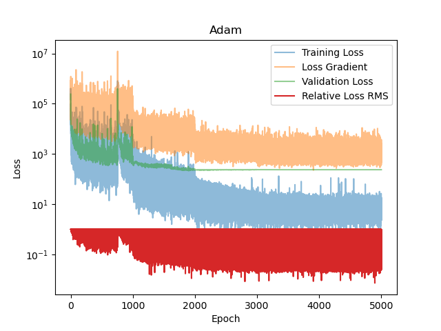
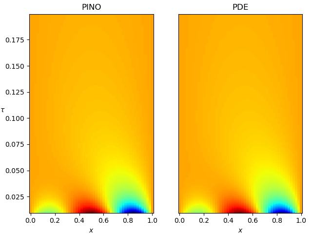
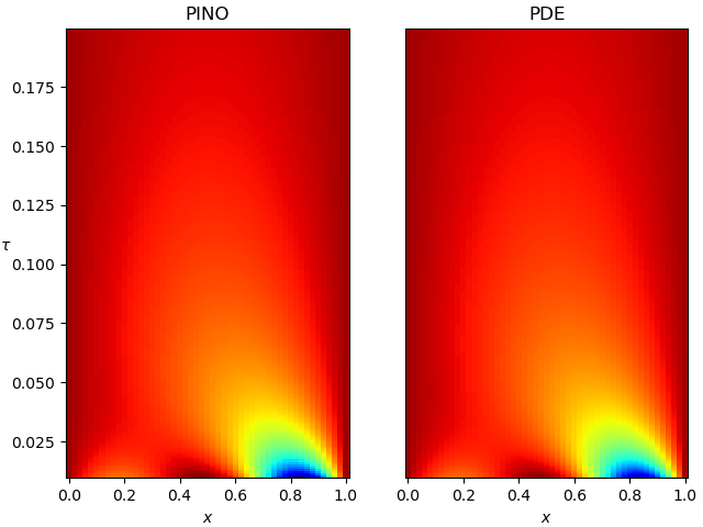
So how does this model perform? Figure 2 shows a heat map of the PDE solution, obtained by finite differences, and the PINO solution on the same scale. The correspondence is … not great. Sure, the global evolutions match, but the fine-grained structure is off, especially in the initial exponential decay.
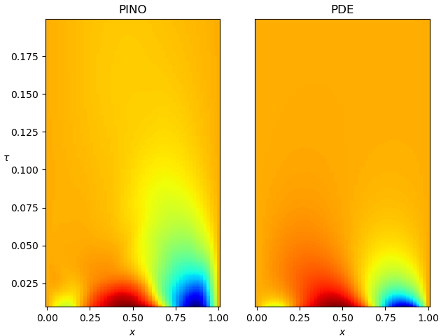
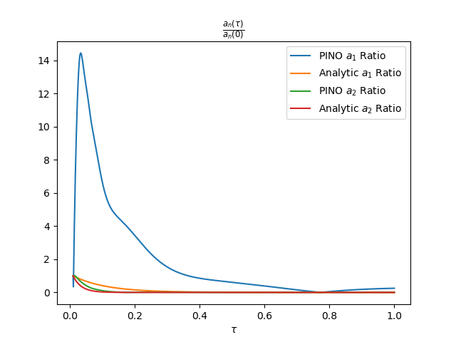
To see this mismatch more clearly, we look at the first Fourier modes. There is a lot of beautiful theory about the diffusion equation, known as the field of harmonic analysis. One result is that the Fourier coefficients
\[a_n(\tau) = 2 \int_{0}^1 (T(x, \tau) - T_s) \sin( n \pi x) dx \tag{2}\]decrease exponentially at a rate
\[\frac{a_n(\tau)}{ a_n(0) } = \exp\left(-n^2\pi^2 \tau\right) \tag{3}\]Any decent PINO should be able to follow this rate decay closely, at least when $\tau$ is small. One look at Figure 3 shows that there is a big mismatch. This error is mainly due to the stagnation in the validation loss. Long story short: the network is over-training on the training data and not learning the physics.
Biasing towards smaller $\tau$
The network struggles for small $\tau$, which is where most of the dynamics of the PDE takes place. A standard remedy is to simply add more small values of $\tau$ in the training (and validation) set. Importantly, this biasing does not change the inductive bias of the network - the model is still constrained to learn the underlying physics - but is simply provided with more informative data in the regime where the dynamics are most sensitive. Here we generate $\tau$-values via
\[\log(\tau) = \log(\tau_{\min}) + \left(\log(\tau_{\max}) - \log(\tau_{\min})\right) u^{\gamma}, \quad u \sim \mathcal{U}[0,1], \tag{4}\]with $\gamma = 2$. When $\gamma > 1$ the distribution of $\tau$ will be largely skewed towards small values = exactly what we need. $\tau_{\min}$ is just a small value to avoid dealing with the log of zero. I use $\tau_{\min}=10^{-3}$. $7000$ out of $10000$ samples for $\tau$ are generated using (4), and $30\%$ are uniform between $0$ and $\tau_{\max}$ to still keep some large training samples so the network doesn’t ‘forget’ long-time evolution.
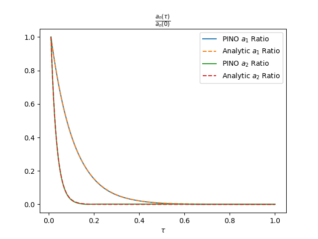
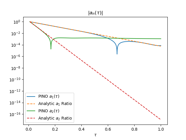
Figure 4 shows the resulting predictions in Fourier space. The learned Fourier modes closely follow the expected exponential decay, indicating that the PINO captures the correct spectral structure of the solution. The figure on the right displays the same Fourier modes in log scale. We see that the decay rate indeed matches initially, but small residual oscillations and mild discrepancies appear once $\tau > 0.6$. These deviations are quantitatively minor and occur in a regime where the dynamics are already strongly damped, but they highlight the remaining limitations of the model at long time scales. Nevertheless, Figure 5 shows an excellent match of the PDE solutions!
Resolving Large $\tau$: Trying a Deeper Network
The current network only has two hidden layers with $64$ neurons each. This is probably right on the edge for this example. A deeper network should theoretically translate to more expressiveness, decreased loss and fit on the real PDE solution. Here I try a network with 4 hidden layers and 64 neurons per layer. The dataset and training routine are the same as in the previous section.

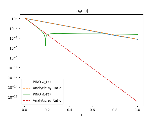
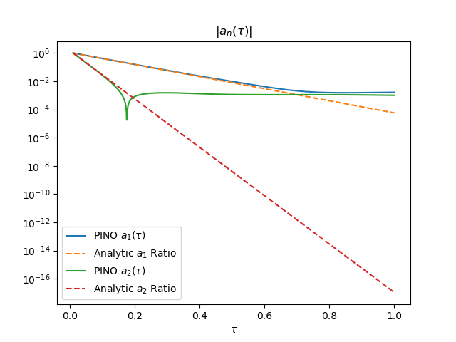
Figure 6 shows the Fourier coefficients of the deeper MLP in log-scale - and we see they follow the analytic coefficients for much longer in time, indicating improved training! This figure also showcases another aspect of PINNs. PINNs generally learn the low-frequency components of the solution well but tend to underperform on the high-frequency modes. The reason is simple: PINNs/PINOs optimize the physics residual, not the fit on the solution. Minimizing the latter would be ideal - it is the solution we are interested in after all - but analytic solutions are generally not available (what would be the point of PINNs otherwise?) so we have to do the best possible job with only the physics residual.
Resolving Large $\tau$: Regularization (Weight Decay)
A final technique to avoid the superfluous oscillations in the first Fourier mode of Figure 4 (still the network with only two hidden layers) is weight decay or $L_2$ regularization. Weight decay adds a term
\[\frac{1}{2} \lambda w^Tw\]to the physics loss to penalize large weights. Large weights typically induce non-physical oscillations in PINNs, so maybe it can also help us here. Some researchers might call these oscillations overfitting, but I don’t think that term applies here. The network is not overfitting on particular samples $\tau_b, \log \kappa_b, T_{s,b}$ but learns an oscillation that is not physical.
Regularization adds another hyperparameter, $\lambda$, to the learning problem. Determining the optimal $\lambda$ has been an area of deep research, and a lot of compute is spent on finding it because it is a problem-dependent setting. A good rule of thumb is that the regularization term should be $5\%$ to $10\%$ of the total loss. We use $\lambda = 10^{-6}$ here.
Interestingly, regularization makes the Fourier modes worse - see Figure &. $a_1(\tau)$ flattens after $\tau>0.7$. This makes sense since we limit weight variability, so we are also limiting the expressiveness of the network.
Perhaps regularization does not cooperate with physics.
Discussion and Conclusion
Figure 8 compares the best-performing PINO model (the 4-layer network) and the true PDE solution obtained by finite differences (different color scheme and parameters compared to Figures 2 and 5). The agreement is excellent: the dominant spatial structure, the transient dynamics at small $\tau$, and the long-time decay toward steady state are all captured accurately. This final result confirms that, with the right training setup and inductive biases, physics-informed neural operators the diffusion equation to high fidelity.
I learned many things from these experiments. First, and unfortunately, PINOs are highly sensitive to the distribution of training data, especially in time. Uniform sampling in $\tau$ led to stagnation in validation loss and poor reproduction of the early-time dynamics, where the heat equation exhibits the most rapid changes. Simply biasing the sampling toward smaller $\tau$ values dramatically improved performance, allowing the network to correctly learn the exponential decay rates of the leading Fourier modes.
Second, architectural capacity matters, especially at long times. While a shallow MLP was sufficient to capture the dominant low-frequency behavior of the solution, it struggled to faithfully track the decay of Fourier modes for larger $\tau$. Increasing network depth extended the time horizon over which the learned spectral decay matched the analytic behavior. This aligns with a broader observation in the literature: PINNs learn low-frequency components well but perform poorly on the high-frequency modes.
Finally, regularization does not seem to add much to physics-informed learning. Although weight decay is supposed to suppress spurious oscillations in some settings, and is a great tool to avoid overfitting for classifiers and transformers, it adds a non-physics term to an otherwise physics loss.
In the next leg of my journey I will finally turn to actual operators. Stay tuned!