So far in this series, I have been training physics-informed neural networks to solve increasingly interesting differential equations. These equations have mostly come from classical physics: heat flow and elastic structural deformations. In this post we take a break from regular physics and enter a new arena: quantum physics, molecules, and solving the Schrödinger equation using PINNs!
Readers of my channel will know why I get excited about this topic. I am deeply interested in computational chemistry because of all the promises it holds. Computational chemistry is the gateway to a new era of discovering medicine and designing molecules, chemical compounds, and materials fit for the task. There is still a long way to go, but this future is closer than you realize!
All these tasks rely on seeing chemistry, molecules and quantum physics through the computational lens. To describe any molecular system, we only need two key quantities: the potential‑energy surface of a given configuration and the forces that the atoms exert on one another. If we can compute these accurately and efficiently, we can optimize molecular geometries, simulate molecular dynamics, search for reaction paths, and start asking design questions.
From first principles, these molecular energies come from quantum mechanics. In particular, for a fixed arrangement of atomic nuclei, the electronic wave function satisfies the stationary Schrodinger equation
\[\hat{H} \psi = E\psi. \tag{1}\]| We are interested in two quantities: the electron probability distribution $ | \psi(x) | ^2$ (the wave function squared) and the associated potential energy $E$. |
Don’t be fooled by this innocently-looking equation. It is a nasty second-order PDE in disguise! This post is about whether the physics-informed learning machinery can be pointed at this equation.
The Smallest Molecule in the Universe
Even for very simple atomic configurations, the Schrödinger equation is a beast to solve. It seems like PINNs actually have an edge over traditional solvers here. In this post we will solve the stationary Schrödinger equation for $H_2$ in three dimensions. $H_2$ is the smallest molecule imaginable that doesn’t just consist of one atom.
This is where the math gets a lot more complicated because we can’t talk about the Schrödinger equation without also introducing some quantum mechanics. PINNs have a surprising connection to a fundamental principle in quantum mechanics. Feel free to skip the rest of this section if you’re only interested in the machine learning part!
Consider the $H_2$ molecule. Let’s assume the positively charged nuclei $H^+$ are located in fixed positions $R_1 = (-R, 0, 0)$ and $R_2 = (R, 0, 0)$ at a distance $d = 2R$ apart. We denote the position of the electron by $r = (x,y,z)$. The positively charged protons repel and build up an electrical energy of $1/d = 1/(2R)$ between them. The electron is delocalized and its wve function $\psi$ satisfies the stationary Schrödinger equation
\[-\frac{1}{2}\nabla^2 \psi(r) + \left(\frac{1}{|r-R_1|}+\frac{1}{|r-R_2|}\right) \psi(r) = E \psi(r) \tag{2}\]The whole left-hand side can be identified with the Hamiltonian $\hat{H} \psi(x)$. The first term is the Laplacian (sum of second derivatives) of the wave function, the second term measures the electric potential energy between the electron and both nuclei
\[V(r) = \frac{1}{|r-R_1|}+\frac{1}{|r-R_2|}.\]| Even for this simple system, the Schrödinger equation is already very complicated. The $1/ | r-R_1 | $ terms create a lot of (computational) complexity. |
There are many great ways of solving this equation in the literature. Most methods boil down to discretizing the PDE in some way and turning it into a matrix eigenvalue problem. These approaches definitely work, but they are expensive and very involved. Physics-informed learning has an edge over traditional methods for solving (2), though there are some immediate issues. First, second-order derivatives of $\psi$ are expensive to evaluate. With PINNs, the PDE is the loss function and one would need to calculate second derivatives of every batch. Second, the energy level $E$ is not a priori known so the PDE is not closed.
Fortunately, both issues can be solved at once by transferring to the weak form of the PDE. Solving (2) is equivalent to minimizing the functional
\[\mathcal{E}[\psi] = \frac{\langle \psi \mid \hat{H} \mid \psi \rangle}{\langle \psi \mid \psi \rangle}. \tag{3}\](Apologies for the sudden appearance of Dirac notation) $\mathcal{E}[\psi]$ measures the energy of the electron, through its wave function. If you’re unfamiliar with Dirac notation,
\[\langle f \mid g \rangle = \int f(r) g(r) dr\]is the inner product between the functions $f$ and $g$. Using the divergence theorem, we can expand (3) into
\[\mathcal{E}[\psi] = \frac{ \int \frac{1}{2} |\nabla \psi(r)|^2 - V(r) |\psi(r)|^2 dr }{\int |\psi(r)|^2 dr}, \tag{4}\]which removes the second derivative! The weak formulation is mathematically identical to the Schrödinger equation but has become easier to evaluate for PINNs. This solves our first issue. Second, the weak form (4) can be used directly as the neural network loss instead of the PDE (2). Miraculously, the right-hand side energy value $E$ has disappeared in the weak formulation. In fact, the ‘ground state’ energy will just pop out as a result of training the PINN,
\[E = \underset{\psi}{\min} \ \mathcal{E}[\psi].\]A huge numerical win!
This is a big deal. Training the physics-informed neural network is equivalent to computing the ground-state energy of the electron (for fixed nuclei). This connects directly to a fundamental idea in quantum chemistry: the Born-Oppenheimer approximation. In this approximation, the nuclei are held fixed while the electron relaxes to its minimal-energy state. The energy of the molecule is then the electronic ground-state energy plus the direct repulsion between the nuclei. In our example of two hydrogen atoms with one electron, the total molecular energy is therefore
\[E_{\text{total}} = \frac{1}{2R} + \underset{\psi}{\min} \ \mathcal{E}[\psi]. \tag{5}\]To all you quantum purists out there, this formula for the total energy is not at all correct because there are many other fundamental interactions at play. Fixing the nuclei probably doesn’t make much physical sense but it provides a nice mental picture. Please cover your ears and shut off your quantum brain for the rest of this post - PINNs is really where the action is at!
Schrödinger’s PINN
Welcome back everyone.
The goal of this post is really to train a physics-informed neural network for an important partial differential equation. If you’ve skipped the previous section, our setup is straightforward: design a physics-informed architecture for solving the Schrödinger equation for $H_2$ by minimizing the energy loss (4). The architecture is very simple: a multilayer perceptron with $4$ inputs, $x, y, z$ and $R$, and just one output, $\psi(x,y,z)$. There is no need to add fancy branch and trunk layers, embedding, conditioning, etc. because there is nothing else in our setup. The physics, and therefore the PINN, is just a $4 \to 1$ map.
There is one more element (pun not intended) needed to make this idea work, and that is evaluating the physics loss / electron energy (4). The physics loss is really an aggregate of the wave function $\psi(r)$ over the entire physical domain. In practice we can’t evaluate that integral exactly (our $\psi$ is a black box), so we have to approximate it numerically. This leaves one choice: grid-based integration versus Monte Carlo methods.
With a grid‑based integration you hand the network the same set of $r_i=(x_i,y_i,z_i)$ coordinates (collocation points) over and over again. This introduces a big risk of overfitting because the network can learn to memorize those particular points rather than learn the underlying physics. The Monte Carlo method draws points at random, forcing the network to generalize. The loss evaluations become noisy, but that isn’t really a problem. Stochastic gradients are a feature; they help the network learn and generalize faster for the same reasons as mini-batching. I won’t dive into the Monte Carlo details here, but you can see the implementation in the code on GitHub if you’re curious.
Some Pretty Pictures
Can PINNs learn the Schrödinger equation? We trained the physics-informed network described in the previous section using the Adam optimizer where the learning rate decreases from $10^{-3}$ to $10^{-6}$ over $1500$ epochs. At each epoch, we sample $B = 256$ values of $\log R$ uniformly, as well as $N=5000$ Monte Carlo particles $(x,y,z)$. As validation metric, we calculate the electron energy for $R = 1$, which has a definite theoretical value of $-1.1030$ Hartree. If the PINN generalizes well, it should reach this minimal energy up to some tolerance.
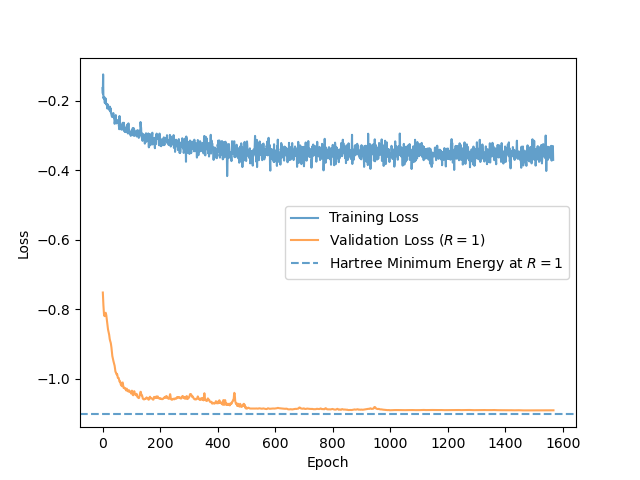
Figure (1) shows the training and validation loss as training progresses. The PINN doesn’t quite reach the Hartree energy, but it’s a great first approximation! The actual probability density, the squared wavefunction, has sharp peaks at the nuclei, where the Coulomb attraction is strongest, and then decreases. However, the PINN is unable to recover these sharp peaks because its output is a differentiable function of its inputs. The network captures the broad, low-frequency structure of electron orbital well, but struggles with the ‘cusps’ at the nuclei. Still, it is surprising that we can reach the ground-state energy so closely while getting the wave function substantially wrong!
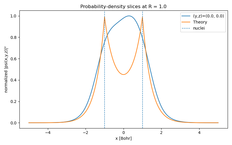
Instead, we need to help the PINN to represent these peaks. Since the locations of the nuclei are fixed and known, we can put the exponentials directly into the network output with a learnable decay parameter $\alpha$
\[\psi(x) = \left(1-\frac{|r|^2}{r_{\text{cutoff}}^2}\right) \left(e^{-\alpha|r - R_1|} + e^{-\alpha|r - R_2|} \right) \text{NN}_{\theta}(r, R). \tag{6}\]| The exponential terms provide the correct qualitative behavior near the nuclei and make it much easier for the network to recover the sharp peaks in the probability density. In theory, $\alpha \approx 1$ but we don’t want to give away too much of the juice! The prefactor $1- | r | ^2 / r_{\text{cutoff}}^2$ comes from our (artificial) Dirichlet boundary conditions at $r = r_{\text{cutoff}}$. |
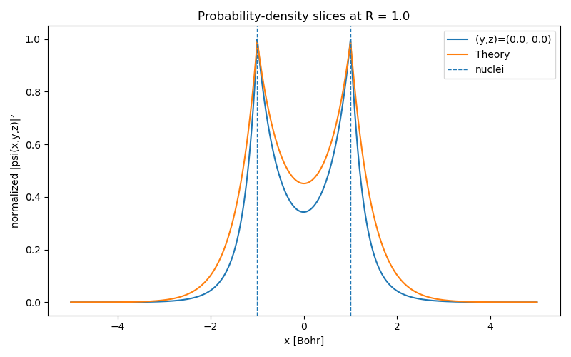
This new ansatz works remarkably well! The resulting probability density (Figure (3)) now closely follows the envelope-based reference (remember, this is not the exact probability!), and the predicted electronic energy improves to $-1.1032$ Hartree, a near-exact match. The tiny remaining difference (notice our energy is smaller) is likely due to Monte Carlo noise.
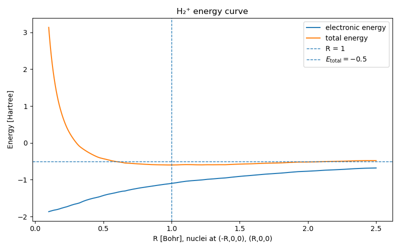
The real litmus test for any computational method is how well it can reproduce the total molecular “binding” energy curve as a function of $R$ — half the distance between the two protons. In the Born‑Oppenheimer picture the binding energy is simply the sum of the proton‑proton Coulomb repulsion and the electronic ground‑state energy (5). In Figure (4) we show the electron ground-state energy and total molecular energy, computed by the physics-informed network, as a function of $R$. We reproduce the classical attraction-repulsion curve of the hydrogen bond!
When the two nuclei are very close together, $R \to 0$, the proton–proton electric repulsion blows up and dominates the total energy. The atoms really want to move away from each other in this state. As the protons are pulled apart, the electron has more space to move and has a lower energy, but the attractive interactions between the electron and the nuclei also fade. At very large distances $R \to \infty$, the electron roams freely but feels no attraction anymore, so its energy goes to zero. There is no net binding between the two protons.
Between these two extremes lies a sweet spot: at $R=1$ the repulsive Coulomb force and the electron attraction balance and the molecule reaches a minimum in the total energy. In theory, that minimum marks the equilibrium bond length.
Next Steps
It is important not to assign any deep quantum insights to these results - they are only as accurate as the Born-Oppenheimer approximation and the expressiveness of the neural network. Still, it is remarkable to me that PINNs can solve the Schrödinger equation accurately and predict electron ground-state and binding energies.
These results make me wonder how far we can push these ideas. Could PINNs be trained to predict the two-electron ground state of $H_2$? What about other atoms like helium, lithium, nitrogen, oxygen, can we predict their ground-state energies through physics-informed learning? The quantum chemistry tends to get a lot more complicated once more than one electron is involved at the same time, but perhaps there is a beautiful mechanism to enforce parity and symmetry straight into the network?
These are all just open questions, and we won’t answer any of them right now, yet it is interesting that we are approaching the realm of machine-learning potentials (MLPs - I know…). This is currently a hot topic in the computational chemistry world! The aim of machine learning potentials is to predict the total molecular energy and forces of any configuration of atoms. They are often trained in a data-driven way from existing quantum chemistry calculations. Their promise is that they can predict quantum-accurate energies and forces much faster than running full quantum simulations.
PINNs are the other side of the coin: they are trained from first principles (quantum) physics, and as we’ve demonstrated here, they can predict energies accurately. It seems to me that physics-informed learning can take a central place in the computational chemistry landscape.
Let’s find out together!