PDE-constrained optimization provides a rigorous framework for optimizing functionals subject to partial differential equation (PDE) constraints. It is one of those techniques that appears deceptively simple from a distance but actually becomes increasingly subtle and complicated once you dive into the details. It is one of the greatest tools that modern computational science has to offer, yet few people truly understand the underlying mathematics and complexity. While PDE-constrained optimization is most commonly associated with shape and topology optimization, its potential for control, design, and yield optimization in physical and chemical systems is, in my view, significantly underappreciated.

In this blog post I explain the mathematics of PDE-constrained optimization in detail, with a special focus on the adjoint method for calculating gradients of the objective function. I also demonstrate an implementation using FEniCS and dolfin for maximizing the yield of a gaseous $\text{CO}_2$ to $\text{O}_2$ reactor.

The Variational Formulation

Let’s start from a time-independent partial differential equation

where $u(x)$ is the solution and $p \in \mathbb{R}^m$ is a set of parameters. We will assume that any forcing terms and boundary conditions have already been incorporated in this formulation. Time-independence is not strictly necessary — one might be interested in minimizing the maximal value of $\lVert u(x,t)\rVert$ over $t$ — but it does make the upcoming derivation somewhat easier.

In most situations, the PDE is already discretized prior to optimization. Let $x = {x_i}_{i=1}^N \in \mathbb{R}^{dN}$ be the nodes or grid points and $u = (u(x_1), u(x_2), \dots, u(x_N)) \in \mathbb{R}^{dN}$. Then the condition that the PDE must be satisfied in the grid points becomes

where $F:\mathbb{R}^{dN}\times\mathbb{R}^m\to\mathbb{R}^{dN}$ is a nonlinear function. It is very common to use PDE-constrained optimization in conjunction with the finite element method, in which case equation (2) coincides with the weak form of the PDE. The objective is to optimize a scalar functional $J(u,p): \ \mathbb{R}^{dN}\times\mathbb{R}^m\to\mathbb{R}$ of the solution $u$ and the parameters $p$. I will focus on minimization, but maximization can be treated equivalently. We solve

Note that we can already make a simplification here. For a given parameter value $p$, the PDE has only one solution (in theory, multiple solutions are possible near folds or bifurcation points, in which case the solution is unique locally). This means it is possible to write the solution as a function $u=u(p)$. The constrained problem (3) reduces to

and the optimum occurs whenever

The reduction from a constrained to an unconstrained formulation simplifies the optimization procedure a lot. Given the current parameter guess $p_n$, we:

• Solve the discrete PDE $F(u,p_n)=0$ for $u(p_n)$;
• Evaluate $f(p_n)=J(u(p_n),p_n)$;
• Somehow compute the gradient $\frac{df}{dp}(p_n)$;
• Pass the objective and its gradient to an optimizer to compute $p_{n+1}$.

This is all there is to PDE-constrained optimization: a gradient-based optimizer running on top of a PDE solver. Typical choices are Newton, (L-)BFGS, or gradient descent (often with Adam).

The Adjoint Method

The hard part is computing the gradient

Here, $\partial J/\partial u \in \mathbb{R}^{Nd}$ is a row vector of partial derivatives of the objective with respect to the solution, and $\partial J/\partial p\in\mathbb{R}^m$ is usually easy to compute The difficult term is the Jacobian

which measures how the PDE solution changes with the parameters. There are two main approaches to computing such sensitivities: automatic differentiation (AD) and finite differences. Most large-scale legacy PDE solvers are not compatible with AD, especially when they rely on black-box solvers or iterative linear algebra routines. Differentiable PDE solvers are a very recent research topic.

As a result, one typically resorts to finite differences. The idea is to perturb each component of $p$ by $\varepsilon e_i$ and solve the PDE:

Then the $i$-th column of the Jacobian is approximated by

This is extremely expensive: it requires solving the PDE $m$ times. Since the PDE solve is usually the computational bottleneck, this approach quickly becomes impractical.

The Lagrangian

Fortunately, we do not need the full Jacobian $du/dp$ — only its action on $\partial J/\partial u$. Since $F(u(p),p)=0$ for all $p$, differentiating with respect to $p$ gives

or equivalently,

Substituting into (6) yields

This expression is still problematic because it involves the inverse of the PDE Jacobian. To avoid this, we introduce the Lagrangian

where $\lambda\in\mathbb{R}^{Nd}$ is the adjoint variable. A classical result from optimization theory is that critical points of $\mathcal{L}$ correspond to critical points of $J$ under the PDE constraint.

Taking the derivative with respect to $u$ gives the KKT condition:

Plugging this into (9) leads to a remarkable simplification:

The expensive inverse has vanished. We now have a gradient formula depending only on how $F$ and $J$ depend on $p$.

The Adjoint Equation

We still need to compute $\lambda$. From (11) we obtain the adjoint equation:

This is a linear system with the same dimension as the original PDE discretization. It is usually well-posed and can be solved with standard numerical linear algebra techniques.

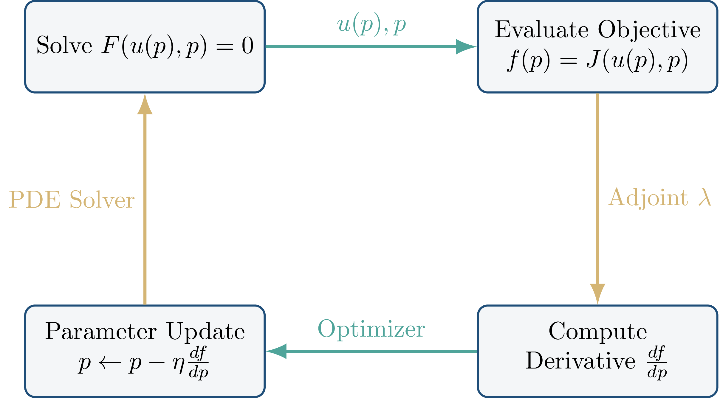
In summary, PDE-constrained optimization proceeds in four steps:

1. Solve the primal PDE for $u(p)$.
2. Solve the adjoint PDE (13) for $\lambda$.
3. Compute the gradient using (12).
4. Update $p$ with any gradient-based optimizer.

This makes adjoint methods dramatically more efficient than finite differences when $m$ is large. These steps are also shown on Figure 1.

A Note on Implementation

The main computational challenge is forming the adjoint matrix $\left(\partial F/\partial u\right)^T$. Once it is available, solving the adjoint system is routine.

Modern finite element libraries like FEniCS can construct this matrix automatically using algorithmic differentiation (“taping”). This is one of the reasons FEniCS has become a standard tool for PDE-constrained optimization.

Conclusion

PDE-constrained optimization is one of the most powerful tools in modern computational science. From wind turbine blades to airplane wings to chemical reactors, many engineering problems can be formulated within this framework — yet the underlying mathematics is often underappreciated.

This post provided a compact mathematical explanation of the adjoint method for efficient gradient computation. I hope you found it useful for your work.