Operator Learning: The Right Way

Over the last week, I have taken a hands-on deep dive into operator learning for the heat equation. Boy, it has been a frustrating journey; and we are far from done. I can’t remember the last time I have had these many ups and downs in my professional life, and it has only been five days!

The goal of this post is to summarize my findings on how to do proper physics-informed operator learning. Along the way, I will also discuss practical lessons learned, common failure modes, and design choices that materially affect performance. In particular, I want to introduce Feature-wise Linear Modulation (FiLM) for physics-informed learning.

In case you’re struggling with PINNs and PINOs, I just want to say: don’t despair. All the details need to be right before the physics-informed model will even start to train. They’re very picky that way. I hope you find this post helpful.

Recap: PINNs for the Heat Equation

We started this journey with the simplest possible physics-informed setup: Newton’s law of cooling

which served as a clean sanity check for physics-informed learning. We trained a model that learned the thermal evolution $T(t)$ for any initial temperature $T_0$, rate constant $\kappa$ and heat bath temperature $T_s$. In many ways, this ML model was already a neural operator, not a simple PINN, because it works for any parameter setting. Newton’s heat law is a low-dimensional, well-conditioned dynamical system. The ODE residual is cheap to evaluate, the gradients are stable, and the optimization landscape is relatively smooth.

In my last post, we moved on to the one-dimensional diffusion (heat) equation

with a fixed initial temperature profile $T_0$. Compared to the ODE, this equation presents a serious shift in complexity. In particular, the learning problem becomes significantly stiffer due to the existence of multiple spatial Fourier modes, each decaying at a rate proportional to $\exp(-\kappa k^2 t)$. Small time scales (small $t$ or small $\tau=k t$) dominate the dynamics, and errors there propagate throughout the solution. Unfortunately, the loss landscape becomes highly irregular and we had to pull a lot of tricks out of the hat to make the PINO learn the physics!

Here is a short summary of the magic tricks required to make stiff PINOs converge: (1) Include as much physics as possible into the network; normalize any dimensional variables, for example $u(x,t)=(T(x,t)-T_s)/T_{\max}$; (2) bias the data generation of all variables towards regions of high stiffness; (3) Make the network deep enough. An MLP with four hidden layers and $100$ neurons per layer may sound like a lot of parameters for learning a simple PDE, it is necessary to get the higher-frequency modes right. More about this point later.

The First Actual Operator

Today we increase the complexity even more by learning a PINO that gives the solution for any initial condition

A random initial condition is not just some extra input parameter like $\kappa$ or $T_s$. We need to feed an entire function to the neural network, a totally different mathematical object. Going back to the physics, this presents a large increase in difficulty because most of the dynamics occurs at small $t$, in other words, close to the initial condition. The PINO must become much more expressive to handle the extra complexity.

One question that plagued me for some time is why we need to include the initial condition in the network at all? Remember we include the initial (Dirichlet) condition in the network output via

with $\tau = k t$ and $g_{\theta}$ the actual input-output function of the neural network. Does this formulation alone take care of $u_0$? Not really. The analytic solution of the heat equation is

where $a_n$ are the Fourier modes of $u_0$. That is, the whole time evolution depends on the initial condition, not just the first time point. The neural operator will essentially learn the first few Fourier coefficients to predict the time evolution - so it must be an input.

Sampling Initial Conditions with Gaussian Processes

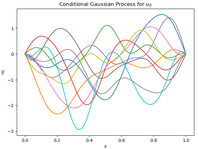
To probe the generalization capabilities of neural operators, we sample initial temperature profiles $u_0(x)$ from a Gaussian process (GP). A GP defines a rich distribution over smooth functions that satisfy the prescribed Dirichlet boundary conditions. With this class of initial conditions, the PINO is encouraged to learn the actual underlying solution operator to the PDE instead of overfitting on a small number of crafted initial conditions. So, theoretically, the learned PINO can predict the temperature evolution of any smooth initial function.

In this example, the Gaussian process is a joint Gaussian distribution with zero mean and a squared-exponential covariance kernel

where the correlation length $\ell$ controls the smoothness and typical spatial scale of variations in the initial condition. In practice, small $\ell$ emphasizes high-frequency structure, while large $\ell$ produces slowly varying profiles. Technically, we use a conditional GP because $u_0$ must satisfy the Dirichlet boundary conditions. Figure 1 shows a few sample functions.

So how do we pass a function to a neural network? The classic trick is to discretize $u_0(x)$ in fixed grid points

and pass the discretized vector $(u_{0,0}, u_{0,1}, \dots, u_{0,N})$ as extra inputs to the neural network. This idea is often known as grid-based physics learning and is in contrast to geometry-agnostic learning. For reference, I will use $N = 51$ grid points in this post.

Two Global Architecture Alternatives

Simply adding $51$ extra input neurons to the network is unlikely to work well, mainly because these inputs are treated as being “equally important” as the other four: $x, t, \log \kappa$, and $T_s$. Moreover, the $51$ grid values do not contain independent information: typical initial conditions are smooth, so $u_0$ varies slowly across adjacent grid points and lives in a much lower-dimensional ‘effective space’ than $\mathbb{R}^{51}$. Naively concatenating $u_0$ therefore introduces redundancy, poor conditioning, and an unnecessarily hard learning problem.

In this post, I explore two underused approaches for incorporating initial conditions (or, more generally, functional inputs like source terms) into neural operators

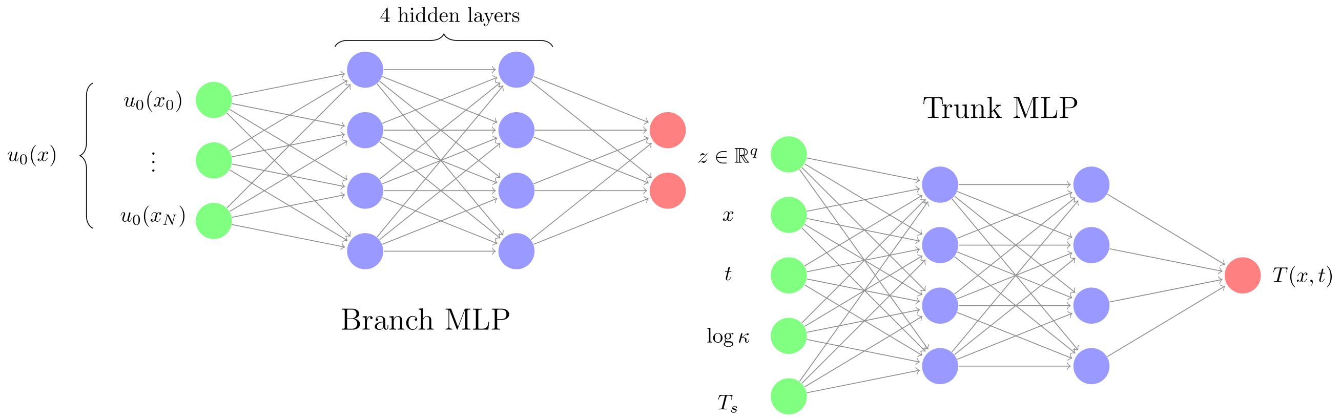
• Low-dimensional embedding via a branch network: map $u_0$ to a compact latent representation $z \in \mathbb{R}^q$ with $q < 51$, and feed this embedding as additional inputs to the main (trunk) network. Figure 2 (a) displays this network architecture;
• Feature-wise Linear Modulation (FiLM): inject information from $u_0$ into each layer of the trunk network via learned, input-dependent affine transformations. FiLM produces an immensely powerful representation and has helped me previously with diffusion models for science. Figure 2 (b) displays this network architecture.

The terms “branch” and “trunk” follow the standard nomenclature introduced in the DeepONet literature. The branch network encodes functional inputs or conditioning variables (here, the initial condition $u_0$), while the trunk network (typically smaller) operates on space and time $(x, t)$. I do not keep to these strict definitions here; the rate constant $\kappa$ and the ambient temperature $T_s$ are fed directly into the trunk network alongside $x$ and $t$. I think the important distinction is point-wise conditioning (trunk) versus global conditioning (branch), not conditioning versus physics.

Let’s delve deeper into the branch network. It’s input (the initial condition) contains a lot of spatial dependence. In this way, it shares many of the characteristics of images. Images are also mostly smooth except for sharp lines or corners. This observation has led SciML researchers to use convolutional layers in the branch network. They use it all the time, but somehow rarely seem to mention it in their writings. Convolutions exploit locality, making them have a much more natural inductive bias for processing functions than fully connected layers. Convolutional layers are forced to interpret neighboring inputs as points that are close in physical space, which is exactly what we need. For an MLP, adjacent input neurons are just that: fully independent.

Indeed, let’s see what happens when we refine the spatial discretization from $N$ points to $2N$. The MLP input layer needs to double in size, meaning twice as many weights and biases in the first layer. In fact, the number of neurons in the subsequent layers will likely need to increase somewhat too to avoid compressing all spatial information in the first layer. On the other hand, convolutions layers do not need to get bigger because they only use local operations - they don’t care whether the input has grid size $\Delta x$ or $\Delta x / 2$. The MLP approach may work sufficiently well when the number of grid points is small - like in the current example - but there will come a point when scaling favors convolutions.

Convolutional Layers are Essential for Functions It took me a few days to fully appreciate how important convolutional networks are for processing functions. Don’t get me wrong, plain MLPs work on discretized initial conditions, they work well for $N=51$, but this setup is fundamentally misaligned with the structure of the data. Convolutional networks provide much better inductive bias. I make this point concrete below using the heat equation as a running example.

Branch-MLP + Trunk-MLP Let’s start from the same trunk network structure as last time, a simple neural network with four hidden layers and 64 neurons / features per layer. The inputs are $(x, t, \log \kappa, T_s)$. All these inputs are normalized to improve training. In the baseline branch approach, the initial condition $u_0(x)$ (also normalized to make dimensionless) is fed directly into a fully connected branch network

with $q = 32$. After passing $z$ through a LayerNorm, this lower-dimensional embedding is then concatenated to the four original inputs, i.e. $(x, t, \log \kappa, T_s, z)$ and passed to the trunk network

Combined, the trunk network has 36 inputs (4 + 32).

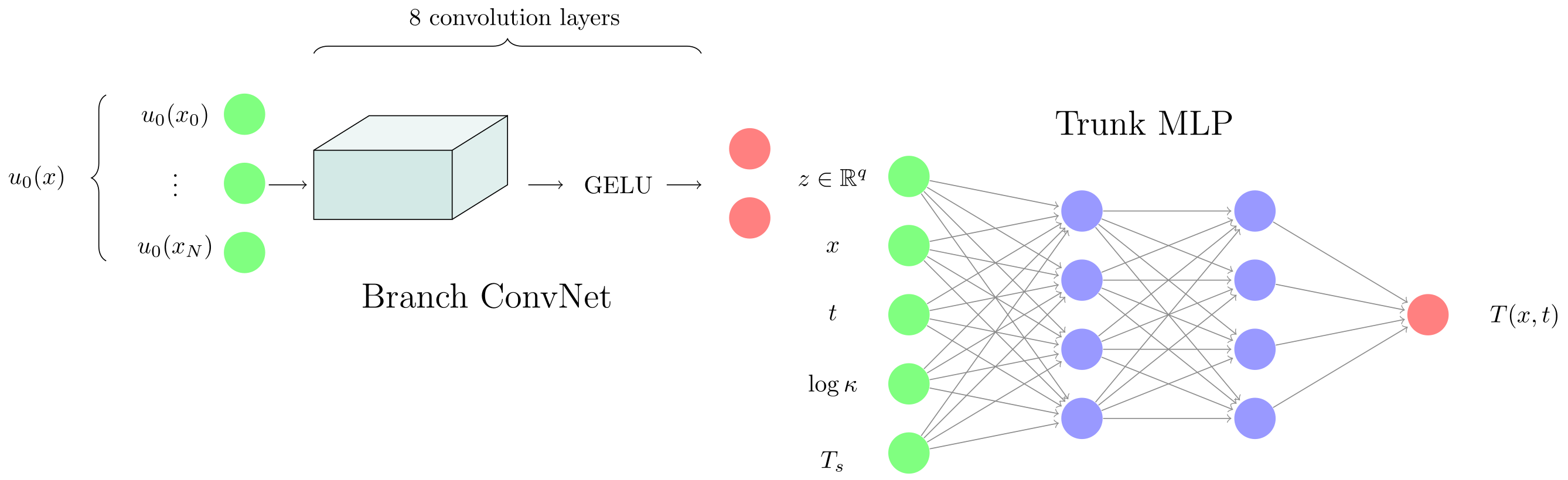
Convolutional Branch Network In the convolutional approach, each linear layer is replaced by a convolutional layer that uses a small local filter ( with a typical kernel of size $3$, $5$ or $7$ - we use $5$ ) to process the data. Per ‘channel’, the convolutional layer only needs to learn $5$ parameters (ignoring the bias). As a result, convolutions are much more parameter efficient! This efficiency is enabled by enforcing physical continuity, an underappreciated point.

However, learning one convolution kernel (also known as a channel) is hardly enough to process random input functions. We use $32$ channels and a total of $8$ back-to-back convolution layers in our Conv-Branch setup. The total ‘width’ of the network is $5 \times 8$ (kernel size x number of layers), meaning every point can see 40 neighbors after 8 layers - enough the process the full physical field ($40 \approx 51$ grid points). At the end of these convolution layers, the output has shape $(B, 32, 51)$ and we use average pooling to reduce this to $(B, 32)$ before passing to the trunk (with another LayerNorm).

For comparison, the branch-MLP approach uses 32,865 trainable parameters, while the Conv-Branch setups use 50,413 trainable parameters. Figure 1 shows both architectures.

Both neural networks are trained using the Adam optimizer with an initial learning rate of $10^{-4}$, which is kept constant over $1000$ epochs. Afterwards, the learning rate is decreased gradually to $10^{-6}$ using a cosine annealing scheduler over $10,000$ epochs. During training, we keep track of the loss, loss gradient, validation loss and the root mean-squared error (RMS). The RMS is a metric for how much of the physics the network has learned. I highly recommend checking out my previous post here for explicit formulas of the loss, RMS and neural network network output.

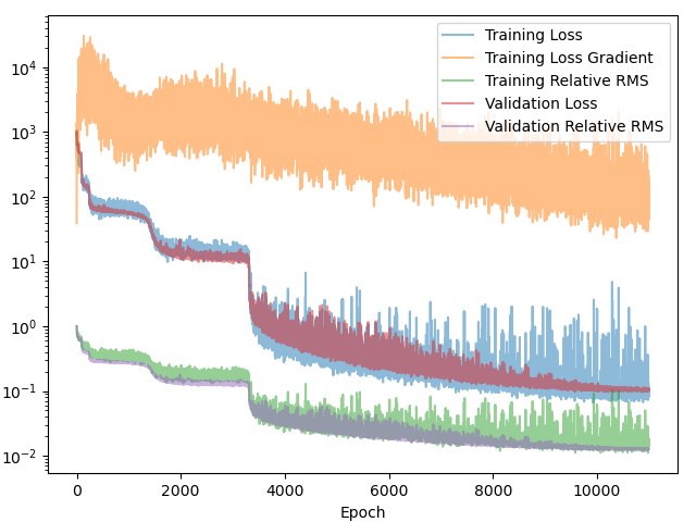
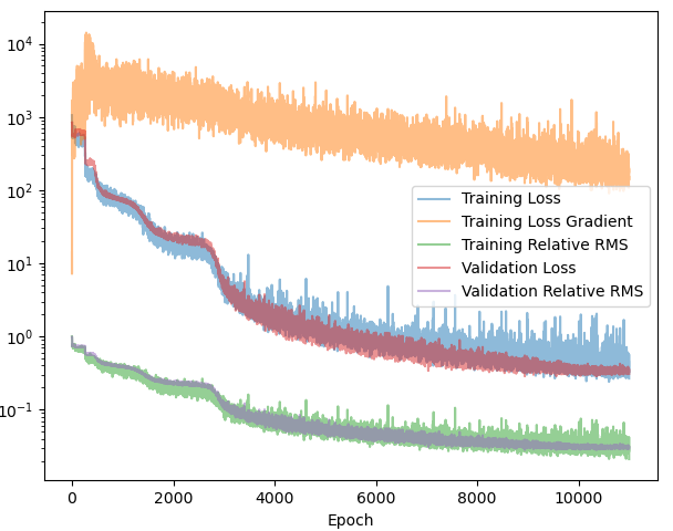
Figure 3 compares the Branch-MLP (left) and Conv-Branch (right) models. Even on a coarse discretization - where an MLP should, in principle, benefit from having global access to the entire function - both models reach essentially the same final performance (loss $\approx 0.1$, RMS error $\approx 1.2\%$). More importantly, the loss curve is slightly smoother on the convolutional side. The MLP tends to stagnate for a while before it ‘discovers’ some more physics. ConvNets have this effect built-in.

The bigger win is in scaling: as the discretization is refined, the convolutional branch continues to work well, while the MLP branch becomes increasingly unwieldy. In practice, this makes convolutional encoders the more scalable and future-proof choice for operator learning.

A Note on Data Sampling and Overfitting Because the branch network is very expressive, training on a fixed and finite set of initial conditions has always led to overfitting. Finally realizing this lifted a huge part of my frustration this week! PINOs require fresh training data to hone in on the underlying physics, ideally every epoch. Overfitting happens mostly branch network; in earlier experiments with a fixed initial condition and a trunk-only architecture, using the same static dataset of $(x, t, \kappa, T_s)$ did not exhibit any overfitting.

Unfortunately, this is a familiar issue in physics-informed learning: the network tends to memorize the residual at specific locations rather than learning the underlying operator. In practice, resampling new functional inputs and space–time points each epoch is a simple but powerful way to encourage genuine physics learning.

This is also why I can’t use second-order optimizers such as L-BFGS. L-BFGS requires a fixed dataset for stable repeated gradient evaluations. To avoid overfitting, one would need a very large static dataset (ideally larger than the number of parameters in the branch network). Unfortunately, the gradient taping graph would blow up my MacBook with only 16 GiB of RAM. The Adam optimizer with small and stochastic batches is the best I can do for this post.

Feature Embedding versus Feature-wise Modulation

Although embedding a lower-dimensional representation of the initial condition works well for our example, it is not the most expressive neural network architecture we could use. I recently worked with another approach to conditioning on input variables in the context of diffusion models. Read about it here if you are interested.

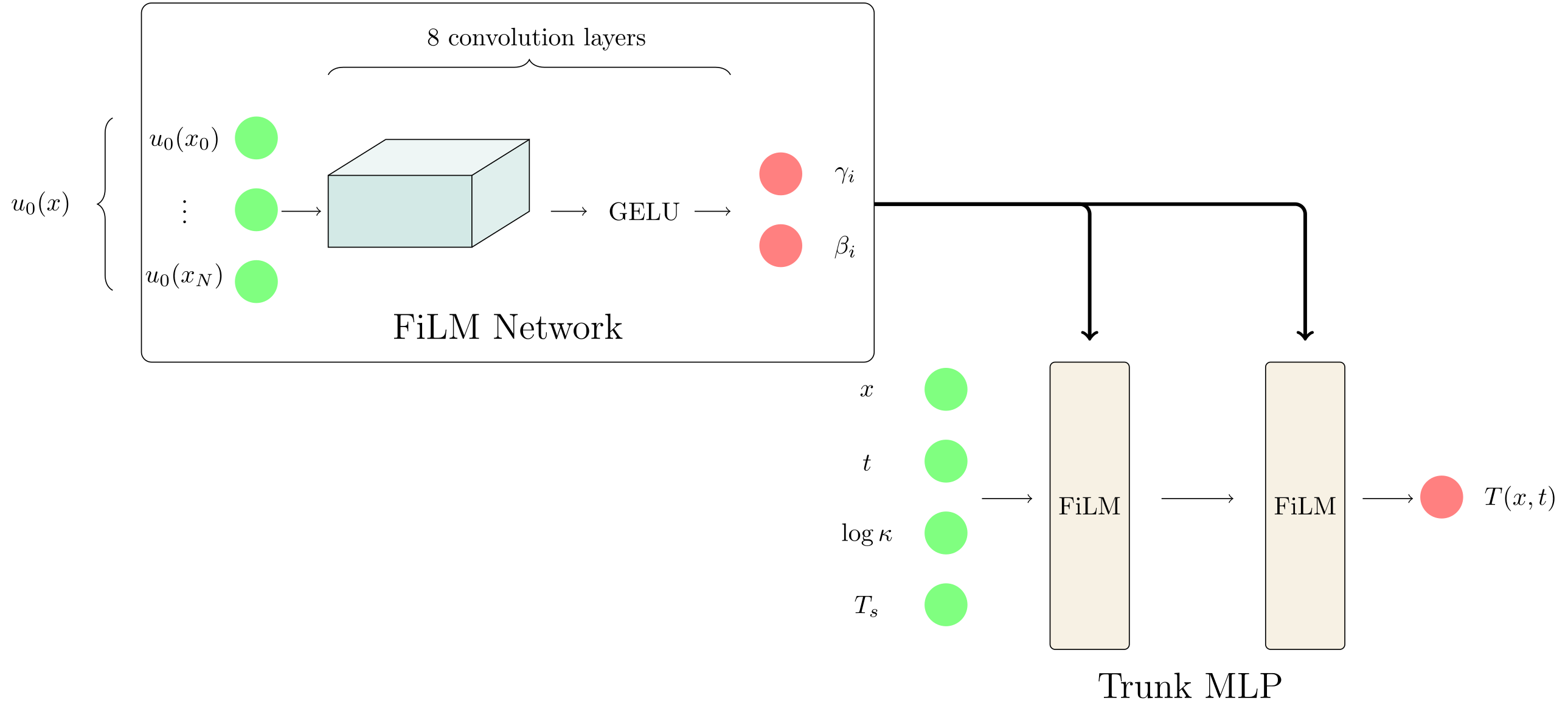
This alternative approach is based on Feature-wise Linear Modulation (FiLM) - a very powerful technique. Feature-wise Linear Modulation uses the same convolutional backbone to encode $u_0$, but instead of producing a single global embedding, it outputs a pair of modulation vectors $(\gamma_i, \beta_i)$ for each layer $i$ of the trunk network. If $z_i \in \mathbb{R}^{64}$ denotes the pre-activation output of the $i$-th linear layer in the trunk network, FiLM applies an input-dependent affine modulation before the nonlinearity,

where the product $\gamma_i z_i$ is taken element-wise over the features of $z_i$. Consequently, both $\gamma_i$ and $\beta_i$ must have the same dimensionality as $z_i$ (here, 64). See Figure 4 for a visual representation of the FiLM operator.

FiLM does not compress the initial condition into a global low-dimensional latent code. Instead, it conditions the trunk network through a collection of layer-wise, high-dimensional modulation parameters $(\gamma_i, \beta_i)$, one pair per trunk layer. This increased expressiveness of the conditioning mechanism tremendously compared to a global embedding, at the cost of additional learnable parameters. In our setup, this increases the parameter count to $117,345$ from $50,413$ for the branch-MLP baseline.

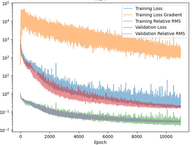
Figure 5 shows the training progress of the FiLM-PINO model. While it reaches the same final loss and root mean-squared error as the embedding-based approach, the optimization trajectory is markedly smoother and exhibits far less of the characteristic “staircase” behavior. This suggests that FiLM provides a better-conditioned optimization problem, likely due to the more expressive, layer-wise conditioning of the trunk network. Based on this behavior, I expect FiLM-style conditioning to generalize more robustly to more complex settings. In fact, it already has for scalar conditioning variables in my prior work. My hypothesis is that FiLM will become the conditioning tool for functions too.

Some Pretty Pictures

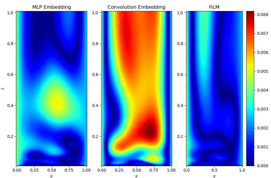
Finally, I want to show a visual comparison between the embedding-based approaches (both MLP and convolutional branch) and FiLM conditioning. All three models reach comparable final losses and RMS errors, but they arrive there in noticeably different ways. The figures below show representative solution profiles and error maps for identical test initial conditions and parameter settings.

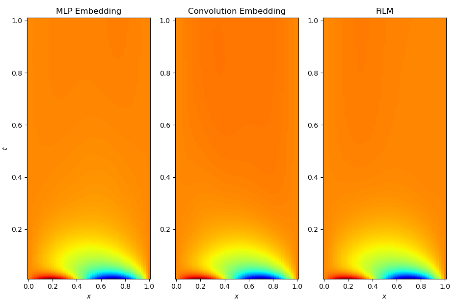
While the embedding-based models tend to capture the large-scale structure of the solution well, subtle discrepancies appear in regions with sharp gradients and during early-time dynamics. In contrast, the FiLM-conditioned model produces visibly smoother and more accurate solution profiles across space and time, with fewer localized artifacts. This qualitative difference is consistent with the smoother optimization behavior observed during training and supports the view that layer-wise conditioning provides a more expressive and better-conditioned way of injecting functional information into the network.

Next I want to look at an example that has been bugging me for months: Neumann boundary conditions for an elliptic PDE. Stay tuned!